Method for Finding the Exact Effective Hamiltonian of Time-Driven Quantum Systems
Author
Alejandro Kunold
Title
Method for Finding the Exact Effective Hamiltonian of Time-Driven Quantum Systems
Description
This program calculates the evolution operator of a Paul trap using the power of Lie algebras as explained in DOI: 10.1002/andp.201900035
Category
Academic Articles & Supplements
Keywords
Lie algebras, quantum evolution operator
URL
http://www.notebookarchive.org/2021-02-3qtrfek/
DOI
https://notebookarchive.org/2021-02-3qtrfek
Date Added
2021-02-08
Date Last Modified
2021-02-08
File Size
244.4 kilobytes
Supplements
Rights
Redistribution rights reserved

Quantum harmonic oscillator with time-dependent frequency
Quantum harmonic oscillator with time-dependent frequency
supplement to: DOI: 10.1002/andp.201900035
Modules
Modules
Thefollowingmodulesrefertothealgebra={,...,},thatfulfilsthecommutationrule,=iℏ,characterizedbythestructureconstants
ℒ
n
h
1
h
n
h
i
h
j
∑
=1
c
i,j,k
h
k
c
i,k,j.
LieGetMa
LieGetMa
LieGetMa[c,J,vα]generatestheMtransormationsofthefor=fork=1,...,nand=...isann×nmatrixandMisann×n×ntensorcorrespondingtothestructureconstantsc.
M
k
-
Q
k
e
M
n+1
M
1
M
n
◼
c : n×n×n tensor containing the structure constants,
◼
J :n×nmatrix,h'=Jhisanewrepresentationofthe
ℒ
n
◼
vα:dimensionnlistvα={,,...,}containingthetransformationparametersforthetransformation.
α
1
α
2
α
n
U
A
LieGetMa[c_,J_,vα_]:=Module[{dim,k,Q,M},dim=Dimensions[c][[1]];k=Dimensions[J][[1]];M=Table[0,{k1,1,k+1},{k2,1,dim},{k3,1,dim}];M[[k+1]]=IdentityMatrix[k];Do[Q=Table[Sum[c[[k2,k3,k4]]J[[k1,k2]]vα[[k1]],{k2,1,dim}],{k3,1,dim},{k4,1,dim}];M[[k1]]=MatrixExp[-Q];M[[k+1]]=M[[k+1]].M[[k1]];,{k1,1,k}];M]
LieGetNu
LieGetNu
LieGetNu[M,J] generates the ν matrix where ν is an n×n matrix.
◼
M : n×n×n tensor containing the transformation matrices,
◼
J:n×nmatrix,h'=Jhisanewrepresentationofthe.
ℒ
n
LieGetNu[M_,J_]:=Module[{dim,Mk,Ik,νt,νt1},dim=Dimensions[M[[1]]][[1]];Ik=Normal[SparseArray[{{1,1}1},dim]];νt1=Ik.J;Do[Mk=M[[k1]];Ik=Normal[SparseArray[{{k1,k1}1},dim]];νt=νt1.Mk+Ik.J;νt1=νt;,{k1,2,dim}];Transpose[νt]]
LieTrans
LieTrans
LieTrans[M,J,va,vα,k,t]transformsthecoeficientsIintova'underthek'thtransformationcorrespondingtothematrix.UnderthistransformationtheoriginalFloquetoperatorH-=h-istransformedintoH'-=(H-)=h--=h-whereva' isthenewsetofcoefficients.
U
k
M
k
p
t
⊤
va
p
t
p
t
U
k
p
t
U
k
⊤
va
M
k
α
k
h
k
p
t
⊤
(va')
p
t
◼
M : n×n×n tensor containing the transformation matrices,
◼
J:n×nmatrix,h'=Jhisanewrepresentationofthe,
ℒ
n
◼
va:dimensionnlistva={,,...,}containingthecoefficientsoftheoriginalFloquetoperator,
a
1
a
2
a
n
◼
vα:dimensionnlistvα={,,...,}containingthetransformationparametersforthetransformation,
α
1
α
2
α
n
U
A
◼
k : integer that tags the number of transformation to be used,
◼
t : time parameter.
LieTrans[M_,J_,va_,vα_,k_,t_]:=va.M[[k]]-D[vα[[k]],t]J[[k]]
LieGetu
LieGetu
LieGetu[M,J,va,vα,t]transformstheoriginalcoefficientsvaintouunderthecompletetransformationcorrespondingto=....UnderthistransformationtheoriginalFloquetoperatorH-=istransformedintoH'-=(H-)=h--=h-.
U
A
M
a
M
1
M
2
M
n
p
t
va.h-p
t
p
t
U
A
p
t
U
A
⊤
va
M
a
⊤
α
⊤
ν
h
k
p
t
⊤
u
p
t
◼
M : is an n×n×n tensor containing the transformation matrices,
◼
J:n×nmatrix,h'=Jhisanewrepresentationofthe,
ℒ
n
◼
va:dimenisonnlistva={,,...,}containingthecoefficientsoftheoriginalFloquetoperator,
a
1
a
2
a
n
◼
vα:dimensionnlistcontainingthetransformationparametersforthetransformation.Theαparametersmustbefunctionsofthetimeparametert.
U
A
◼
t : time parameter.
LieGetu[M_,J_,va_,vα_,t_]:=Module[{k,vu,vw},k=Dimensions[vα][[1]];vu=va;Do[vw=LieTrans[M,J,vu,vα,k1,t];vu=vw;,{k1,1,k}];vu]
LieGetDifEqLambda
LieGetDifEqLambda
LieGetDifEqLambda[J,νi,vα,vβ,λ,ci] calculates a list containing
the differential equations with respect to the auxiliary parameter
λ that connects the α and β parameters.
the differential equations with respect to the auxiliary parameter
λ that connects the α and β parameters.
◼
J:n×nmatrix,h'=J.hisanewrepresentationofthe,
ℒ
n
◼
νi : inverse of the n×n matrix ν calculated with LieGetNu[M,J],
◼
vα:dimensionnlistvα={,,...,}containingthetransformationparametersforthe.Theαparametersmustbefunctionsoftheauxiliaryparameterλ,
α
1
α
2
α
n
U
A
◼
vβ:dimensionnlistvβ={,,...,}containingthetransformationparametersforthe.TheβparametersareNOTfunctionsoftheauxiliaryparameterλ,
β
1
β
2
β
n
U
B
◼
λ : is the auxiliary parameter that helps relate the α and β transformation parameters.
◼
ci:isaBooleanvariable.IfciTrue,theinitialconditions[0]0,[0]0,...,[0]0isappendedtothelistofdifferentialequations.IfonciFalsethentheoutputisjustthelistofdifferentialequations,
α
1
α
2
α
n
◼
λ : is the auxiliary parameter that helps relate the α and β transformation parameters.
LieGetDifEqLambda[J_,νi_,vα_,vβ_,λ_,ci_]:=Module[{dim,v},dim=Dimensions[vα][[1]];v=νi.vβ;If[ciTrue,Join[Table[D[vα[[k1]],λ]v[[k1]],{k1,1,dim}],Table[(vα[[k1]]/.λ0)0,{k1,1,dim}]],Table[D[vα[[k1]],λ]v[[k1]],{k1,1,dim}]]]
LieGetNAlpha
LieGetNAlpha
LieGetNAlpha[J,νi,vβ,m] numerically calculates the α parameters using Eq. (16).
◼
J:n×nmatrix,h'=J.hisanewrepresentationofthe,
ℒ
n
◼
νi : inverse of the n×n matrix ν calculated with LieGetNu[M,J], νi must be a function of vα.
◼
vα:dimensionnlistvα={,,...,}containingthetransformationparametersforthe.
α
1
α
2
α
n
U
B
◼
vβ:dimensionnlistvβ={,,...,}containingthetransformationparametersforthe.
β
1
β
2
β
n
U
B
◼
m : number of iterations.
LieGetNAlpha[J_,νi_,vα_,vβ_,m_]:=Module{dim,vα0,vα1,cond,νi0},dim=Dimensions[vβ][[1]];vα0=Table[0,{k1,1,dim}];Docond=Table[vα[[k1]]vα0[[k1]],{k1,1,dim}];νi0=νi/.cond;vα1=νi0.vβ+vα0;vα0=vα1;,{m1,0,m-1};vα1
1
m
Main Program
Main Program
Definition of the structure constants ci,j,k
Definition of the structure constants
c
i,j,k
The elements of this algebra are given by the operators =, =xp+px,=. The following lines define the algebra dimension and the structure constants.
h
1
2
x
h
2
h
3
2
p
n=3;d=Table[0,{k1,1,n},{k2,1,n},{k3,1,n}];d[[1,2,3]]=2;d[[2,1,3]]=-2;d[[1,3,1]]=4;d[[3,1,1]]=-4;d[[2,3,2]]=-4;d[[3,2,2]]=4;R={{1,0,0},{0,0,1},{0,1,0}};Ri=Inverse[R];c=Table[Sum[R[[k1,m1]]R[[k2,m2]]Ri[[m3,k3]]d[[m1,m2,m3]],{m1,1,n},{m2,1,n},{m3,1,n}],{k1,1,n},{k2,1,n},{k3,1,n}];
Since J=ℐ, the structure of the algebra elements is preserved.
J=IdentityMatrix[n];
Derivation of the time differential equations for αi(t)
Derivation of the time differential equations for (t)
α
i
We calculate using Eq. (13). Notice that in this case vα = {(t),...,(t)} is a function of time.
α
1
α
n
vα=Table[Subscript[α,k1][t],{k1,1,n}];va=Table[Subscript[a,k1],{k1,1,n}];Ma=LieGetMa[c,J,vα];vu=LieGetu[Ma,J,va,vα,t];Simplify[vu]
-4[t]+4[t]-[t],-2[t]+2[t]-4[t]+4[t]-[t]-[t],+4[t]-4[t]+4[t]-[t]+4[t](-2[t]-[t])-[t]
4[t]
α
2
a
1
a
2
α
1
a
3
2
α
1
′
α
1
a
2
a
3
α
1
4[t]
α
2
α
3
a
1
a
2
α
1
a
3
2
α
1
′
α
1
′
α
2
-4[t]
α
2
a
3
4[t]
α
2
2
α
3
a
1
a
2
α
1
a
3
2
α
1
′
α
1
α
3
a
2
a
3
α
1
′
α
2
′
α
3
Compare these results with the ones in Eqs. (36)-(38).
The simplified differential equations for(t) are obtained from Eq. (15)
The simplified differential equations for
α
i
ν=LieGetNu[Ma,J];νi=Inverse[ν];ℰ=Simplify[νi.vu];difeqst=Join[Table[ℰ[[k1]]0,{k1,1,n}],Table[(vα[[k1]]/.{t0})0,{k1,1n}]];MatrixForm[difeqst]
a 1 a 2 α 1 a 3 2 α 1 ′ α 1 |
a 2 a 3 α 1 ′ α 2 |
-4 α 2 a 3 ′ α 3 |
α 1 |
α 2 |
α 3 |
Compare these results with the ones in Eqs. (40)-(42).
Relation between α(t) and β(t) via the solution of the λ differential equations
Relation between α(t) and β(t) via the solution of the λ differential equations
Using Eq. (17) we workout the λ differential equations for the (λ,t) parameters. Note that in this case vα = {(λ),...,(λ)} is a function of λ therefore, andνhavetoberecalculated. In LieGetDifEqLamda the condition ci is set to False in order to avoid setting the initial conditions.
α
i
α
1
α
n
M
a
vα=Table[Subscript[α,k1][λ],{k1,1,n}];Ma=LieGetMa[c,J,vα];ν=LieGetNu[Ma,J];νi=Inverse[ν];vβ=Table[Subscript[β,k1],{k1,1,n}];difeqsλ=Simplify[ExpToTrig[LieGetDifEqLambda[J,νi,vα,vβ,λ,False]]];MatrixForm[difeqsλ]
(Cosh[4 α 2 α 2 β 1 ′ α 1 |
β 2 β 1 α 3 ′ α 2 |
β 3 β 1 2 α 3 β 2 α 3 ′ α 3 |
Compare these results with Eqs. (26)-(28).
These equations are simple enough that we can attempt to solve them with DSolve, however, as mentioned above it is easier to solve the system without initial conditions.
These equations are simple enough that we can attempt to solve them with DSolve, however, as mentioned above it is easier to solve the system without initial conditions.
sol=Simplify[DSolve[difeqsλ,vα,λ][[1]]]
[λ]+,[λ]C[2]+LogCos2(λ+C[1])[λ]C[3]+(Cosh[4C[2]]-Sinh[4C[2]])Tan2(λ+C[1])
α
3
β
2
-+
Tan2(λ+C[1])2
β
2
β
1
β
3
-+
2
β
2
β
1
β
3
2
β
1
α
2
1
2
-+
,2
β
2
β
1
β
3
α
1
1
2
-+
2
β
2
β
1
β
3
β
1
-+
2
β
2
β
1
β
3
Setting λ=1 we can obtain a relation between α(t) and β(t) of the form (18).
vα1=Table[Subscript[α,k1],{k1,1,n}];eqs=Table[vα1[[k1]]((vα[[k1]]/.sol)/.{λ1}),{k1,1,n}]
C[3]+(Cosh[4C[2]]-Sinh[4C[2]])Tan2(1+C[1])C[2]+LogCos2(1+C[1])+
α
1
1
2
-+
2
β
2
β
1
β
3
β
1
-+
,2
β
2
β
1
β
3
α
2
1
2
-+
,2
β
2
β
1
β
3
α
3
β
2
-+
Tan2(1+C[1])2
β
2
β
1
β
3
-+
2
β
2
β
1
β
3
2
β
1
In principle, one could obtain the inverse relations of the form (18), however, it is easier to resort to the eigenvalue one eigenvectors of .
⊤
M
a
Relation between α(t) and β(t) via the eigenvalue one eigenvectors of ⊤Ma
Relation between α(t) and β(t) via the eigenvalue one eigenvectors of
⊤
M
a
Working out the inverse relation between α and β might be difficult in this case given the complexity of the previous equations. Therefore, it is convenient to obtain a relation between α(t) and β(t) by obtaining the eigenvalue one eigenvectors of . There is one eigenvalue one eigenvector.
⊤
M
a
vα=Table[Subscript[α,k1],{k1,1,n}];Ma=LieGetMa[c,J,vα];Mat=Transpose[Ma[[n+1]]];eval=Simplify[Eigenvalues[Mat]];evec=Simplify[Eigenvectors[Mat]];eval[[1]]=Simplify[evec[[1]]]=
ρ
1
β
1
γ
1
ρ
1
1
,,1
α
1
α
3
1-+4
-4
α
2
α
1
α
3
4
α
3
,,
α
1
γ
1
α
3
1-+4
-4
α
2
α
1
α
3
γ
1
4
α
3
γ
1
Compare this last result with the one in Eq. (30).
Exact Solution
Exact Solution
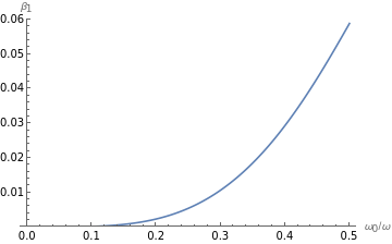
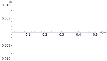
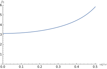
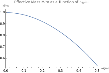
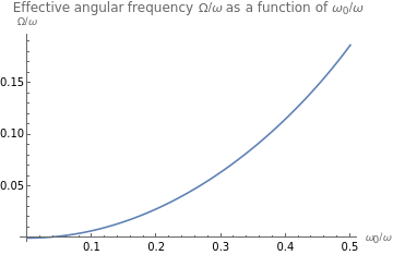
Here we plot the main results concerning the exact solution. Here we used Eqs. (24)-(26), (30) and (32).
MC[ϕ1_,ϕ0_,t_]:=MathieuC[4,-2,t]pMC[ϕ1_,ϕ0_,t_]:=MathieuCPrime[4,-2,t]iMC[ϕ1_,ϕ0_,t_]:=NIntegrate,{s,0,t}
2
ϕ1
2
ϕ0
2
ϕ1
2
ϕ0
1
2
MC[ϕ1,ϕ0,s]
ni=100;qmax=0.5;qmin=0.0005;dataβ1={};dataβ2={};dataβ3={};dataM={};dataΩ={};Doq=qmin+(qmax-qmin)ini;nC0=MC[0,q,0];nC=MC[0,q,π];npC=pMC[0,q,π];niC=iMC[0,q,π];nγ=ArcTan--npCniC+1+--;β1=-nγ;β2=-npCniC-+1nγ;β3=2niCnγ;AppendTo[dataβ1,{q,β1}];AppendTo[dataβ2,{q,β2}];AppendTo[dataβ3,{q,β3}];AppendTodataM,q,;AppendTodataΩ,q,β1-;,{i,0,ni}
4npCniC
2
nC0
nC
2
-npCniC-+1
2
nC0
nC
2
nC0
2
nC
2
nC0
nC
2
nC0
2
nC
4npCniC
2
nC0
nC
2
-npCniC-+1
2
nC0
nC
2
nC0
2
nC
1
2
npC
nC
1
2
2
nC0
nC
2
nC0
2
nC
2
nC0
π
β3
β3
2
π
2
β2
β3
ListPlot[dataβ1,AxesLabel{"/ω",""},PlotRange{0.0,0.06},JoinedTrue]ListPlot[dataβ2,AxesLabel{"/ω",""},PlotRange{-0.01,0.01},JoinedTrue]ListPlot[dataβ3,AxesLabel{"/ω",""},PlotRange{0,6.0},JoinedTrue]ListPlot[dataM,AxesLabel{"/ω","M/m"},PlotLabel"Effective Mass M/m as a function of /ω",JoinedTrue]ListPlot[dataΩ,AxesLabel{"/ω","Ω/ω"},PlotLabel"Effective angular frequency Ω/ω as a function of /ω",JoinedTrue]
ω
0
β
1
ω
0
β
2
ω
0
β
3
ω
0
ω
0
ω
0
ω
0
Numerical Solution
Numerical Solution
First we do some preliminary calculations.
vα=Table[Subscript[α,k1],{k1,1,n}];Ma=LieGetMa[c,J,vα];ν=LieGetNu[Ma,J];νi=Inverse[ν];
To illustrate the numerical method we start by obtaining just one point of the effective Hamiltonian for the quantum harmonic oscillator with time-dependent frequency (Paul trap). This means that the β parameters are calculated for one value of the mass (=1.0) and =2.0. As an example we have chosen ω = 4.0.
H
e
ω
0
m=100;=1.0;ω0=2.0;ω=10.0;T=2π/ω
0.628319
We numerically solve (NDSolve) the time differential euqtions difeqst for the α parameters obtained above for =1.0, =10.0 and ω = 4.0.
ω
0
vαt=Table[Subscript[α,k1][t],{k1,1,n}];difeqstn=difeqst/.Cos[ωt],0,;solt=NDSolve[difeqstn,vαt,{t,0,T}][[1]];
a
1
2
2
ω0
a
2
a
3
1
2
The solution is then used to obtain α(T), the α parameters evaluated in T.
vαT=vαt/.solt/.{tT}
{0.0234735,-0.00795757,0.344456}
To simplify the calculation we find the eigenvalue one eigenvectors of evaluatedinα(T). We use the eigenvalues and eigenvectors calculated in the previous section. To avoid divergencies we multiply the eigenvectors by
⊤
M
a
α
3
evaln=eval[[1]]/.Table[vα[[k1]]vαT[[k1]],{k1,1,n}]evecn=evec[[1]]/.Table[vα[[k1]]vαT[[k1]],{k1,1,n}];ρ=evecn
α
3
1
{0.0234735,1.05328×,0.344456}
-8
10
We calculate α as a function of β using Eq. (103) and verify that the condition (104) is met.
The inverse function in Eq. (18) is calculated by finding the minimum of the χ function for α(T)
The inverse function in Eq. (18) is calculated by finding the minimum of the χ function for α(T)
χ[γ_]:=;γ=Sort[Table[{γ,χ[γ]},{γ,0.45,1.01,0.0005}],#1[[2]]<#2[[2]]&][[1]]vβN=γ[[1]]ρ
2
Norm[vαT-LieGetNAlpha[J,νi,vα,γρ,m]]
{0.9895,7.19231×}
-9
10
{0.023227,1.04222×,0.340839}
-8
10
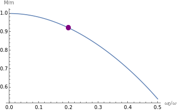
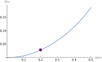
Therefore, for ω=10.0 we have =0.023227,=0.0and=0.340839. To test the numerical solution we can compare it with the previously obtained exact solutions for Ω/ω and M/m as functions of /ω .
β
1
β
2
β
3
ω
0
ListPlotdataM,ω0ω,,PlotStyle{Automatic,Directive[PointSize[0.03],Purple]},Joined{True,False},AxesLabel{"/ω","M/m"}ListPlotdataΩ,ω0ω,/ω","Ω/ω"}
π
ωvβN[[3]]
ω
0
1
π
vβN[[1]]vβN[[3]]
,PlotStyle{Automatic,Directive[PointSize[0.03],Purple]},Joined{True,False},AxesLabel{"ω
0
The reader may change the value of the parameter ω and repeat the calculation to verify that the numerical solution is consisten with the exact one.
Now we add a loop to the procedure to calculate the effective Hamiltonian for various values of the parameter ω.
Now we add a loop to the procedure to calculate the effective Hamiltonian for various values of the parameter ω.
m=100;=1.0;ω0=2.0;ωmin=5.0;ωmax=35.0;Δω=3.0;dataNM={};dataNΩ={};prog=0.0;ProgressIndicator[Dynamic[prog]]Doprog=(ω-ωmin)(ωmax-ωmin);T=2πω;vαt=Table[Subscript[α,k1][t],{k1,1,n}];difeqstn=difeqst/.Cos[ωt],0,;solt=NDSolve[difeqstn,vαt,{t,0,T}][[1]];vαT=vαt/.solt/.{tT};evaln=eval[[1]]/.Table[vα[[k1]]vαT[[k1]],{k1,1,n}];evecn=evec[[1]]/.Table[vα[[k1]]vαT[[k1]],{k1,1,n}];ρ=evecn;χ[γ_]:=;γ=Sort[Table[{γ,χ[γ]},{γ,0.45,1.01,0.0005}],#1[[2]]<#2[[2]]&][[1,1]];vβN=γρ;AppendTodataNM,ω0ω,;AppendTodataNΩ,ω0ω,
a
1
2
2
ω0
a
2
a
3
1
2
α
3
2
Norm[vαT-LieGetNAlpha[J,νi,vα,γρ,m]]
π
ωvβN[[3]]
1
π
vβN[[1]]vβN[[3]]
;,{ω,ωmin,ωmax,Δω}Superimposing the exact solution for Ω/ω and M/m as functions of /ω, to the numerical one, we obtain the following plot
ω
0
ListPlot[{dataM,dataNM},PlotStyle{Automatic,Directive[PointSize[0.03],Purple]},Joined{True,False},AxesLabel{"/ω","M/m"}]ListPlot[{dataΩ,dataNΩ},PlotStyle{Automatic,Directive[PointSize[0.03],Purple]},Joined{True,False},AxesLabel{"/ω","Ω/ω"}]
ω
0
ω
0
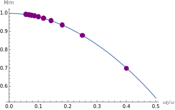
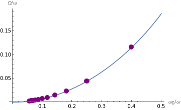
We observe that the numerical solution for the effective Hamiltonian is identical to the exact one.
Cite this as: Alejandro Kunold, "Method for Finding the Exact Effective Hamiltonian of Time-Driven Quantum Systems" from the Notebook Archive (2021), https://notebookarchive.org/2021-02-3qtrfek
Download
