CO2 gradients inside a leaf
Author
Fulton Rockwell
Title
CO2 gradients inside a leaf
Description
State 2 in figures 3&4 Rockwell 2024 New Phytologist https://doi.org/10.1111/nph.20106
Category
Academic Articles & Supplements
Keywords
leaf gas exchange, stomatal conductance, unsaturation
URL
http://www.notebookarchive.org/2024-11-a5d91wg/
DOI
https://notebookarchive.org/2024-11-a5d91wg
Date Added
2024-11-22
Date Last Modified
2024-11-22
File Size
376.18 kilobytes
Supplements
Rights
CC BY 4.0

State 2 in figures 3&4 Rockwell 2024 New Phytologist https://doi.org/10.1111/nph.20106
CO2 gradients inside a leaf
CO2 gradients inside a leaf
Fulton Rockwell
In[]:=
Remove["Global`*"]
State 2
State 2
Dimensional Solution for ci for leaf with top at z=0 and bottom at z=L.
α=characteristic delta c.
a1=first integration constant
a2=second integration constant
Dimensional Solution for ci for leaf with top at z=0 and bottom at z=L.
α=characteristic delta c.
a1=first integration constant
a2=second integration constant
α=characteristic delta c.
a1=first integration constant
a2=second integration constant
The program is written for three independent compartments/areoles, but here we will use the same parameters for 2&3 to reduce the number of independent compartments to 2.
The program is written for three independent compartments/areoles, but here we will use the same parameters for 2&3 to reduce the number of independent compartments to 2.
In[]:=
gu1=.2;gl1=.5;
In[]:=
gu2=.4;gl2=.15;
In[]:=
gu3=.4;gl3=.15;
In[]:=
α1=0.6(*leafareafracareole1*)
Out[]=
0.6
In[]:=
α2=0.2(*leafareafracareole1*)
Out[]=
0.2
In[]:=
α3=1-α1-α2(*leafareafracareole2*)
Out[]=
0.2
In[]:=
Ogu=α1gu1+α2gu2+α3gu3Ogl=α1gl1+α2gl2+α3gl3
Out[]=
0.28
Out[]=
0.36
DImensional parameters from data
DImensional parameters from data
In[]:=
A1=18.510^-6;(*mol/m2/sassimilationwholethickness*)
In[]:=
A2=20.210^-6;A3=20.210^-6;
In[]:=
Atot=α1A1+α2A2+α3A3
Out[]=
0.00001918
In[]:=
cu=390.5*10^-6;(*molco2/molair,actuallyismolefractionnotconcentration*)(*cl=400*10^-6;*)
In[]:=
Δw=7.38/.95/1000(*uppersurfacemolfractiondiffleaftoair*)
Out[]=
0.00776842
In[]:=
ws=34.04/1000(*satleafmolfraction*)
Out[]=
0.03404
In[]:=
wa=ws-Δw
Out[]=
0.0262716
Dimensional parameters non-varying
Dimensional parameters non-varying
In[]:=
L=20010^-6;(*mleafthicknesscotton*)
In[]:=
τ=1;(*tortuosity,path/lengthsquared,maxplausible?*)ϕ=0.5;(*airfraction*)
In[]:=
cD=40.2*2.510^-5;(*molarvolairtimesdiffwatervaporscaledtoco2,molarconductivity*)
Dummy variables for the surface conductances of an areole and comp specific A
Dummy variables for the surface conductances of an areole and comp specific A
In[]:=
gu;(*=0.21/1.6gsuppermol/m2/s*)
In[]:=
gl;(*gs=0/1.6lowermol/m2/s*)
In[]:=
A;
Non-Dimensional parameters
Non-Dimensional parameters
In[]:=
Δc=1.6;(*charmolfracdiff,ifallAdiffusedwholethickness.Small!*)
AτL
ϕcD
In[]:=
cU=;(*uppercuvetteco2versusdropacrossleafifallAdiffusedacrosswholeleaf:say400/40umol*)cL=;BU=;(*ratioofuppergstogforias,say800vs500mmol/m2/s*)BL=;
cu
Δc
cl
Δc
guτL
ϕcD
glτL
ϕcD
Dimensional Solution: CO2 concentration profile in mol/mol for an areole
Dimensional Solution: CO2 concentration profile in mol/mol for an areole
In[]:=
a1=BU-BUcU;
BLBUcU+BUcU+BLcL-0.5BL-1
(BLBU+BU+BL)
In[]:=
a2=;Δc+a1+a2;
BUcU+BLcL-0.5BL+BLBUcU-1
(BLBU+BU+BL)
z^2
2L^2
z
L
In[]:=
c[gu_,gl_,A_]:=EvaluateΔc+a1+a2(*mol/molCO2*)
z^2
2L^2
z
L
Solve for individual areoles leaving cl as variable
Solve for individual areoles leaving cl as variable
In[]:=
ca1=c[gu1,gl1,A1];
In[]:=
ca2=c[gu2,gl2,A2];
In[]:=
ca3=c[gu3,gl3,A3];
In[]:=
dca1=ca1;
∂
z
In[]:=
lowflux1=-dca1/.zL;
ϕcD
1.6τ
In[]:=
dca2=ca2;
∂
z
In[]:=
lowflux2=-dca2/.zL;
ϕcD
1.6τ
In[]:=
dca3=ca3;
∂
z
In[]:=
lowflux3=-dca3/.zL;
ϕcD
1.6τ
In[]:=
highflux1=-dca1/.z0;
ϕcD
1.6τ
In[]:=
highflux2=-dca2/.z0;
ϕcD
1.6τ
In[]:=
highflux3=-dca3/.z0;
ϕcD
1.6τ
Impose constraint of zero net (across all compartments) flux from lower cuvette
Impose constraint of zero net (across all compartments) flux from lower cuvette
In[]:=
sol=FindRoot[{α1lowflux1+α2lowflux2+α3lowflux30},{{cl,cu}}]
Out[]=
{cl0.000259288}
Check mass conservation: total of all fluxes should equal A
Check mass conservation: total of all fluxes should equal A
In[]:=
totalflux=α1lowflux1+α2lowflux2+α3lowflux3+α1highflux1+α2highflux2+α3highflux3;Atot-totalflux/.sol
Out[]=
-1.63054×
-20
10
Plot solutions for ci curves as PPM
Plot solutions for ci curves as PPM
In[]:=
ca1sol=ca1/.sol;
In[]:=
ca2sol=ca2/.sol;
In[]:=
ca3sol=ca3/.sol;
Set plot options for publication
Set plot options for publication
In[]:=
SetOptions[Plot,BaseStyle->{FontFamily->"Times",FontSize18}];
In[]:=
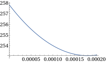
Plot[ca1sol10^6,{z,0,L}]
Out[]=
In[]:=
Plot[ca1sol10^6,{z,0,L},AxesStyleDirective[Black,28],Ticks->{{{.00005,50},{.0001,100},{.00015,150},{.0002,200}},{241,242,243,244,245}},PlotStyle->{Black,Thick},AxesOrigin->{0,239.5},PlotRange->{Full,{239.5,245.5}},AspectRatio->1]
Out[]=

In[]:=
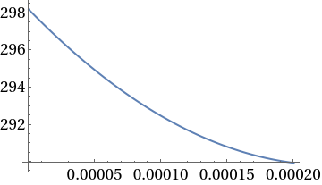
Plot[ca2sol10^6,{z,0,L}]
Out[]=
In[]:=
Plot[ca2sol10^6,{z,0,L},AxesStyleDirective[Black,28],Ticks->{{{.00005,50},{.0001,100},{.00015,150},{.0002,200}},{148,149,150,151,152}},PlotStyle->{Black,Thick},AxesOrigin->{0,147.5},PlotRange->{Full,{147.5,152}},AspectRatio->1]
Out[]=

In[]:=
Plot[ca3sol10^6,{z,0,L}]
Out[]=
Check if ci difference across first areole is positive , in PPM
Check if ci difference across first areole is positive , in PPM
In[]:=
c1l=(ca1sol10^6/.z->L)
Out[]=
253.157
In[]:=
c1u=(ca1sol10^6/.z->0)
Out[]=
257.827
In[]:=
dc1=c1u-c1l
Out[]=
4.67046
Calculate single compartment series model for leaf dCi
Calculate single compartment series model for leaf dCi
In[]:=
Ocu=cu-1.6Atot/Ogu(*Ocuisohmicpredforciu*)
Out[]=
0.0002809
In[]:=
Ocl=cl/.sol(*Ohmicdefassumecil=cl*)
Out[]=
0.000259288
In[]:=
dci=Ocu-Ocl
Out[]=
0.0000216122
In[]:=
dci*10^6(*inPPM*)
Out[]=
21.6122
Rias inferred from CO2 and single compartment model
Rias inferred from CO2 and single compartment model
In[]:=
RiasC=2dci/Atot(*m2s/molDefinitionfromSlatyermodel*)
Out[]=
2.25362
In[]:=
GiasC=1/RiasC
Out[]=
0.443731
In[]:=
RiasW=RiasC/1.6
Out[]=
1.40851
Conserved Rias Ci correction leading to Runsat
Conserved Rias Ci correction leading to Runsat
In[]:=
TargetRtoA=1.55(*,setunderstate1withassumptionofnounsat*)
dci
A
Out[]=
1.55
In[]:=
1.65174
Out[]=
1.65174
In[]:=
CorDci=TargetRtoAAtot
Out[]=
0.000029729
In[]:=
CorOcu=Ocl+CorDci(*Buttheasssumptionthat*)
Out[]=
0.000289017
In[]:=
Corgsc=Atot/(cu-CorOcu)
Out[]=
0.188997
In[]:=
CorOgu=1.6Corgsc
Out[]=
0.302395
In[]:=
wi=Δw+wa
Ogu
CorOgu
Out[]=
0.0334647
Assume same degree of unsat in lower leaf half (this is what Wong et al does...)
Assume same degree of unsat in lower leaf half (this is what Wong et al does...)
In[]:=
CorOgl=Ogl
wi-wa
Δw
Out[]=
0.388794
Define Runsat as the ‘extra’ R required to make Ci based gs match saturated gs, added in series for upper and lower surfaces
Define Runsat as the ‘extra’ R required to make Ci based gs match saturated gs, added in series for upper and lower surfaces
In[]:=
Runsat=1/Ogu-1/CorOgu+1/Ogl-1/CorOgl(*Rh2o-cRh2owaterunits*)
Out[]=
0.470213
Nobel gas comparison: RH is the true aggregate R experienced by noble gas (He) in water units, RU and RL are the true surface resistances.
Nobel gas comparison: RH is the true aggregate R experienced by noble gas (He) in water units, RU and RL are the true surface resistances.
In[]:=
RH=++++++++
-1
-1
1
α1gu1
1
α1gl1
τL
α1ϕcD
-1
1
α2gu2
1
α2gl2
τL
α2ϕcD
-1
1
α3gu3
1
α3gl3
τL
α3ϕcD
Out[]=
8.13515
In[]:=
RU=
-1
(α1gu1+α2gu2+α3gu3)
Out[]=
3.57143
In[]:=
RL=
-1
(α1gl1+α2gl2+α3gl3)
Out[]=
2.77778
Calculating Rias from nobel gas by stripping off stomatal components: true if saturation holds and no series/parallel artifacts
Calculating Rias from nobel gas by stripping off stomatal components: true if saturation holds and no series/parallel artifacts
In[]:=
RiasH=RH-(RU+RL)
Out[]=
1.78594
Summary of Wong calculations as in plot 3a
Summary of Wong calculations as in plot 3a
In[]:=
Rn=RH(*Rseenbynoblegasacrossleafinwaterunits*)
Out[]=
8.13515
In[]:=
Rh2o=RU+RL(*ObservedsurfacetotalRsinserieswithsaturationinsideleaf*)
Out[]=
6.34921
In[]:=
cRh2o=Rh2o-Runsat
Out[]=
5.87899
In[]:=
Rias=Rn-cRh2o
Out[]=
2.25615
In[]:=
Runsat
Out[]=
0.470213
Rias comparisons:
Rias comparisons:
In[]:=
AnatomicalRias=
τL
ϕcD
Out[]=
0.39801
In[]:=
Rias
Out[]=
2.25615
In[]:=
RiasH
Out[]=
1.78594
In[]:=
RiasW
Out[]=
1.40851
In[]:=
dci*10^6(*inPPM*)
Out[]=
21.6122
Cite this as: Fulton Rockwell, "CO2 gradients inside a leaf" from the Notebook Archive (2024), https://notebookarchive.org/2024-11-a5d91wg
Download
