Hu and Mizuno (2020) Mathematica Appendix (5).nb
Author
Qing Hu, Tomomichi Mizuno
Title
Hu and Mizuno (2020) Mathematica Appendix (5).nb
Description
Supplemental notebook to "Endogenous timing and manufacturer advertising: A note"
Category
Academic Articles & Supplements
Keywords
endogenous timing, manufacturer, advertising, vertical market, retailer, pricing
URL
http://www.notebookarchive.org/2020-12-3qctlxw/
DOI
https://notebookarchive.org/2020-12-3qctlxw
Date Added
2020-12-08
Date Last Modified
2020-12-08
File Size
336.24 kilobytes
Supplements
Rights
Redistribution rights reserved

This file contains supplementary data for “Endogenous timing and manufacturer advertising: A note” by Qing Hu and Tomomichi Mizuno.
Endogenous timing and manufacturer advertising: A note
Mathematica Appendix
Endogenous timing and manufacturer advertising: A note
Mathematica Appendix
Mathematica Appendix
Qing and Tomomichi
Faculty of Economics, Kushiro Public University of Economics, Ashino 4-1-1, Kushiro-shi, Hokkaido, 085-8585, Japan. E-mail: huqing549@gmail.com
Graduate School of Economics, Kobe University, 2-1 Rokkodai, Nada, Kobe, Hyogo, 657-8501, Japan. E-mail: mizuno@econ.kobe-u.ac.jp
*
Hu
+
Mizuno
*
+
Clear["Global`*"]
2. Model
2. Model
We define each consumer’s demand as follows.
demand=q1-,q2-
a-p1-aγ+p2γ
b(-1+γ)
a-p2-aγ+p1γ
b(-1+γ)
q1-,q2-
a-p1-aγ+p2γ
b(-1+γ)
a-p2-aγ+p1γ
b(-1+γ)
Since θ consumers watching the advertising, demands for the retailers are
{θq1,θq2}/.demand;Demand={Q1%[[1]],Q2%[[2]]}
Q1-,Q2-
(a-p1-aγ+p2γ)θ
b(-1+γ)
(a-p2-aγ+p1γ)θ
b(-1+γ)
Consumer surplus is
CS=
(--+2(-1+γ)-2a(p1+p2)(-1+γ)+2p1p2γ)θ
2
p1
2
p2
2
a
2b(-1+γ)
(--+2(-1+γ)-2a(p1+p2)(-1+γ)+2p1p2γ)θ
2
p1
2
p2
2
a
2b(-1+γ)
The profits of retailers are
π1=(p1-w)Q1;π2=(p2-w)Q2;
The profit of manufacturer is
πM=(w-c)(Q1+Q2)-(kθ^2);
The producer and total surpluses are
PS=π1+π2+πM;TS=CS+PS;
3. Analysis
3. Analysis
Stage 4: simultaneous pricing
Stage 4: simultaneous pricing
First, we consider the case with simultaneous pricing.From the first-order condition, we obtain in (1).
B
p
{π1,π2};%/.Demand;Solve[{D[%[[1]],p1]0,D[%[[2]],p2]0},{p1,p2}]//Flatten;OutcomepB=%
p1-,p2-
a+w-aγ
-2+γ
a+w-aγ
-2+γ
Stage 4: sequential pricing
Stage 4: sequential pricing
Next, we consider the case with sequential pricing.From the first-order condition, we obtain the best response for the in (2):
F
p
L
p
π2;%/.Demand;Solve[D[%,p2]0,p2]//Flatten;OutcomepF=%;%/.{p1pL}
p2(a+w-aγ+pLγ)
1
2
Then, the leader chooses the price in (3):
L
p
π1;%/.Demand;%/.OutcomepF;Solve[D[%,p1]0,p1]//Flatten//Simplify;OutcomepL=%
p1
w(-2-γ+)+a(-2+γ+)
2
γ
2
γ
2(-2+)
2
γ
Stage 3
Stage 3
Proof of Lemma 1
Proof of Lemma 1
Under simultaneous pricing in the retail market, the manufacturer chooses the following wholesale price.
πM;%/.Demand;%/.OutcomepB;Solve[D[%,w]0,w]//Flatten//Simplify;Outcomew=%
w
a+c
2
Under sequential pricing, the manufacturer sets the following wholesale price.
πM;%/.Demand;%/.OutcomepF;%/.OutcomepL;Solve[D[%,w]0,w]//Flatten//Simplify
w
a+c
2
Hence, we obtain Lemma 1. Q.E.D.
Stage 2
Stage 2
Proof of Lemma 2
Proof of Lemma 2
Under simultaneous pricing in the retail market, the first-order condition leads to the advertising level in (4):
B
θ
πM;%/.Demand;%/.OutcomepB;%/.Outcomew;Solve[D[%,θ]0,θ]//Flatten//Factor;OutcomeθB=%θ/.%;θB=%
θ-
2
(a-c)
4bk(-2+γ)
-
2
(a-c)
4bk(-2+γ)
Similarly, for the sequential pricing case, the manufacturer chooses the advertising level in (5):
S
θ
πM;%/.Demand;%/.OutcomepF;%/.OutcomepL;%/.Outcomew;Solve[D[%,θ]0,θ]//Flatten//FullSimplify;OutcomeθS=%θ/.%;θS=%
θ(-8+(-1+γ)γ(4+γ))
2
(a-c)
32bk(-2+)
2
γ
2
(a-c)
32bk(-2+)
2
γ
Here, we compare with .
B
θ
S
θ
θB-θS//Factor
-(-1+γ)(2+γ)
2
(a-c)
2
γ
32bk(-2+γ)(-2+)
2
γ
Therefore, we obtain >. Q.E.D.
B
θ
S
θ
Here, we present the retailers’ profits in the case with simultaneous and sequential pricing as in (6) - (8).
Here, we present the retailers’ profits in the case with simultaneous and sequential pricing as in (6) - (8).
π1;%/.Demand;%/.OutcomepB;%/.Outcomew;%/.OutcomeθB//Simplify;πB=%
4
(a-c)
16k
2
b
3
(-2+γ)
{π1,π2};%/.Demand;%/.OutcomepF;%/.OutcomepL;%/.Outcomew;%/.OutcomeθS//FullSimplify;{πL,πF}=%
(-1+γ)(-8+(-1+γ)γ(4+γ)),-(-1+γ)(-8+(-1+γ)γ(4+γ))
4
(a-c)
2
(2+γ)
1024k
2
b
2
(-2+)
2
γ
4
(a-c)
2
(-4+(-2+γ)γ)
2048k
2
b
3
(-2+)
2
γ
In addition, we obtain the upstream profit and consumer, producer, and total surpluses under simultaneous pricing are as follows.
{πM,CS,PS,TS};%/.Demand;%/.OutcomepB;%/.Outcomew;%/.OutcomeθB//Simplify;{πMB,CSB,PSB,TSB}=%
,-,(-4+3γ),(-5+3γ)
4
(a-c)
16k
2
b
2
(-2+γ)
4
(a-c)
16k
2
b
3
(-2+γ)
4
(a-c)
16k
2
b
3
(-2+γ)
4
(a-c)
16k
2
b
3
(-2+γ)
Those under sequential pricing are as follows.
{πM,CS,PS,TS};%/.Demand;%/.OutcomepF;%/.OutcomepL;%/.Outcomew;%/.OutcomeθS//FullSimplify;{πMS,CSS,PSS,TSS}=%
,(-8+(-1+γ)γ(4+γ))(32+γ(32+γ(-16+γ(-20+γ+3)))),(-8+(-1+γ)γ(4+γ))(64+(-2+γ)γ(2+γ)(-4+γ(17+3γ))),(-8+(-1+γ)γ(4+γ))(160+γ(64+γ(-152+γ(-52+γ(35+9γ)))))
4
(a-c)
2
(-8+(-1+γ)γ(4+γ))
1024k
2
b
2
(-2+)
2
γ
4
(a-c)
2
γ
4096k
2
b
3
(-2+)
2
γ
4
(a-c)
2048k
2
b
3
(-2+)
2
γ
1
4096k
2
b
3
(-2+)
2
γ
4
(a-c)
Stage 1
Stage 1
Proof of Proposition 1
Proof of Proposition 1
We show the following profit ranking in (9).≤<if0.786≤γ<1,≤<if0.375≤γ<0.786,≤<if0<γ<0.375.First, we compare with .
B
π
L
π
F
π
L
π
B
π
F
π
L
π
F
π
B
π
F
π
L
π
πF-πL//Simplify
-(-1+γ)(4+3γ)(-8-4γ+3+)
4
(a-c)
3
γ
2
γ
3
γ
2048k
2
b
3
(-2+)
2
γ
Hence, we have >.
F
π
L
π
Next, we consider-.
Next, we consider
B
π
L
π
πB-πL//Simplify
-(-1+γ)(-32+16γ+48-8-18++)
4
(a-c)
2
γ
2
γ
3
γ
4
γ
5
γ
6
γ
1024k
2
b
3
(-2+γ)
2
(-2+)
2
γ
The sign of - only depends on the term .Hence, the condition for ->0 is as follows.
B
π
L
π
--32+16γ+48-8-18++
2
γ
3
γ
4
γ
5
γ
6
γ
B
π
L
π
-(-32+16γ+48-8-18++);NSolve[%0,Reals]Plot[%%,{γ,0,1},AxesLabel{γ,"-"},LabelStyleDirective[15]]
2
γ
3
γ
4
γ
5
γ
6
γ
B
π
L
π
{{γ-4.24241},{γ0.785753},{γ1.5127},{γ3.57078}}

Then, ->0 if .
B
π
L
π
γ<0.786
Finally, we compare with .
Finally, we compare
B
π
F
π
πB-πF//Factor//Simplify
((-1+γ)(-128+320γ+192-352-64+112-2-7+))2048k
4
(a-c)
2
γ
2
γ
3
γ
4
γ
5
γ
6
γ
7
γ
8
γ
2
b
3
(-2+γ)
3
(-2+)
2
γ
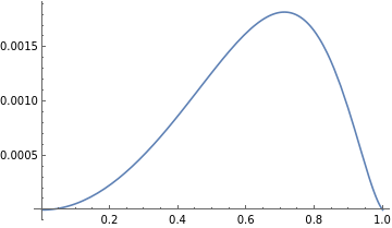
The sign of - only depends on the term .Hence, the condition for ->0 is as follows.
B
π
F
π
--128+320γ+192-352-64+112-2-7+
2
γ
3
γ
4
γ
5
γ
6
γ
7
γ
8
γ
B
π
F
π
-(-128+320γ+192-352-64+112-2-7+);NSolve[%0,Reals]Plot[%%,{γ,0,1},AxesLabel{γ,"-"},LabelStyleDirective[15]]
2
γ
3
γ
4
γ
5
γ
6
γ
7
γ
8
γ
B
π
F
π
{{γ-3.14907},{γ0.375032}}

Then, ->0 if .
Summarizing the above results, we obtain the profit ranking in (9).
From this profit ranking, we directly obtain Proposition 1. Q.E.D.
B
π
F
π
γ<0.375
Summarizing the above results, we obtain the profit ranking in (9).
From this profit ranking, we directly obtain Proposition 1. Q.E.D.
Here, we derive a probability in mixed strategy equilibrium.
Solving+(1-x)=+(1-x) for x, we obtain the following probability.
Here, we derive a probability
x
Solving
B
xπ
L
π
F
xπ
B
π
Solve[xπB+(1-x)πLxπF+(1-x)πB,x]//Flatten//Simplify
x
2(-2+)(-32+16γ+48-8-18++)
2
γ
2
γ
3
γ
4
γ
5
γ
6
γ
256-384γ-448+416+232-132-38+9+
2
γ
3
γ
4
γ
5
γ
6
γ
7
γ
8
γ
FInally, we compare the manufacturer’s profit and the various surplus measures under simultaneous and sequential pricing.
FInally, we compare the manufacturer’s profit and the various surplus measures under simultaneous and sequential pricing.
πMB-πMS//Factor//Simplify%b^2k/(a-c)^4;NSolve[%0,Reals]Plot[%%,{γ,0,1}]
-(-1+γ)(2+γ)(32-18++)
4
(a-c)
2
γ
2
γ
3
γ
4
γ
1024k
2
b
2
(-2+γ)
2
(-2+)
2
γ
{{γ-4.5904},{γ-2.},{γ-1.35127},{γ0.},{γ1.},{γ1.49815},{γ3.44352}}

CSB-CSS//Factor//Simplify%b^2k/(a-c)^4;NSolve[%0,Reals]Plot[%%,{γ,0,1}]
-(-1+γ)(768+384γ-896-384+360+108-58-5+3)
4
(a-c)
2
γ
2
γ
3
γ
4
γ
5
γ
6
γ
7
γ
8
γ
4096k
2
b
3
(-2+γ)
3
(-2+)
2
γ
{{γ-3.63811},{γ-1.31121},{γ0.},{γ1.}}

PSB-PSS//Factor//Simplify%b^2k/(a-c)^4;NSolve[%0,Reals]Plot[%%,{γ,0,1}]
-(-1+γ)(768-384γ-1120+432+528-144-86+11+3)
4
(a-c)
2
γ
2
γ
3
γ
4
γ
5
γ
6
γ
7
γ
8
γ
2048k
2
b
3
(-2+γ)
3
(-2+)
2
γ
{{γ-6.41887},{γ-2.41668},{γ0.},{γ1.},{γ1.02436},{γ3.79742}}
TSB-TSS//Factor//Simplify%b^2k/(a-c)^4;NSolve[%0,Reals]Plot[%%,{γ,0,1}]
-((-1+γ)(2304-384γ-3136+480+1416-180-230+17+9))4096k
4
(a-c)
2
γ
2
γ
3
γ
4
γ
5
γ
6
γ
7
γ
8
γ
2
b
3
(-2+γ)
3
(-2+)
2
γ
{{γ-5.11697},{γ-2.18668},{γ0.},{γ1.},{γ1.31809},{γ1.54455},{γ1.66468},{γ3.61843}}

Therefore, we find that upstream profit and consumer, producer, and total surpluses under simultaneous pricing are higher than those under sequential pricing.
4. Extensions
4. Extensions
4.1. Third-degree price discrimination in wholesale market
4.1. Third-degree price discrimination in wholesale market
Stage 4
Stage 4
First, we consider the case with simultaneous pricing.
In the fourth stage, the first-order condition leads to the following outcomes.
In the fourth stage, the first-order condition leads to the following outcomes.
{π1/.{ww1},π2/.{ww2}};%/.Demand;Solve[{D[%[[1]],p1]0,D[%[[2]],p2]0},{p1,p2}]//Flatten//Simplify;OutcomepBD=%
p1,p2
-2w1-w2γ+a(-2+γ+)
2
γ
-4+
2
γ
-2w2-w1γ+a(-2+γ+)
2
γ
-4+
2
γ
Next, we consider the case with sequential pricing.The follower chooses as follows.
FD
p
j
LD
p
i
π2/.{ww2};%/.Demand;Solve[D[%,p2]0,p2]//Flatten;OutcomepFD=%%/.p2,p1,w2wj
LD
p
j
LD
p
i
p2(a+w2-aγ+p1γ)
1
2
(a+wj-aγ+γ)
LD
p
j
1
2
LD
p
i
The leader sets as follows.
LD
p
i
π1/.{ww1};%/.Demand;%/.OutcomepFD;Solve[D[%,p1]0,p1]//Flatten//Simplify;OutcomepLD=%%/.{p1,w1wi,w2wj}
LD
p
i
p1
-w2γ+w1(-2+)+a(-2+γ+)
2
γ
2
γ
2(-2+)
2
γ
LD
p
i
-wjγ+wi(-2+)+a(-2+γ+)
2
γ
2
γ
2(-2+)
2
γ
Stage 3
Stage 3
Under simultaneous pricing, the manufacturer chooses wholesale prices as follows.
(w1-c)Q1+(w2-c)Q2-kθ^2;%/.Demand;%/.OutcomepBD;Solve[{D[%,w1]0,D[%,w2]0},{w1,w2}]//Flatten//Simplify
w1,w2
a+c
2
a+c
2
Under sequential pricing, the manufacturer sets the following wholesale prices.
(w1-c)Q1+(w2-c)Q2-kθ^2;%/.Demand;%/.OutcomepFD;%/.OutcomepLD;Solve[{D[%,w1]0,D[%,w2]0},{w1,w2}]//Flatten//Simplify
w1,w2
a+c
2
a+c
2
4.2. Timing of advertising
4.2. Timing of advertising
Case (i)
Case (i)
We define the following profits.
π1;%/.Demand;%/.OutcomepB//Simplify;πBT=%
-(-1+γ)θ
2
(a-w)
b
2
(-2+γ)
{π1,π2};%/.Demand;%/.OutcomepF;%/.OutcomepL//Simplify;{πLT,πFT}=%
(-1+γ)θ,-(-1+γ)θ
2
(a-w)
2
(2+γ)
8b(-2+)
2
γ
2
(a-w)
2
(-4-2γ+)
2
γ
16b
2
(-2+)
2
γ
We consider profit ranking.
πFT-πLT//Simplify
-(-1+γ)(4+3γ)θ
2
(a-w)
3
γ
16b
2
(-2+)
2
γ
Hence, we have >.
FT
π
LT
π
πLT-πBT//Simplify
2
(a-w)
4
γ
8b(-2+)
2
(-2+γ)
2
γ
Hence, we have >.
Therefore, we obtain<<.
LT
π
BT
π
Therefore, we obtain
BT
π
LT
π
FT
π
4.3. Persuasive advertising
4.3. Persuasive advertising
We define the following demand functions.
Demandpa=Q1-,Q2-
(a+θ)
b
p1-γp2
b(1-γ)
(a+θ)
b
p2-γp1
b(1-γ)
Q1-+,Q2-+
p1-p2γ
b(1-γ)
a+θ
b
p2-p1γ
b(1-γ)
a+θ
b
We define as follows.
SOC
z
zSOC=1/(2(2-γ))
1
2(2-γ)
Stage 4
Stage 4
Under simultaneous pricing, the first-order conditions yields as follows.
Bpa
p
{π1,π2};%/.Demandpa;Solve[{D[%[[1]],p1]0,D[%[[2]],p2]0},{p1,p2}]//Flatten//Simplify;OutcomepBpa=%%/.{p1,p2}
Bpa
p
Bpa
p
p1,p2
a+w-aγ+θ-γθ
2-γ
a+w-aγ+θ-γθ
2-γ
,
Bpa
p
a+w-aγ+θ-γθ
2-γ
Bpa
p
a+w-aγ+θ-γθ
2-γ
Under sequential pricing, the follower chooses as follows.
Fpa
p
Lpa
p
π2;%/.Demandpa;Solve[D[%,p2]0,p2]//Flatten//Simplify;OutcomepFpa=%%/.{p1,p2}
Lpa
p
Fpa
p
p2(a+w-aγ+p1γ+θ-γθ)
1
2
(a+w-aγ+γ+θ-γθ)
Fpa
p
1
2
Lpa
p
The leader sets as follows.
Lpa
p
π1;%/.Demandpa;%/.OutcomepFpa;Solve[D[%,p1]0,p1]//Flatten//Simplify;OutcomepLpa=%%/.{p1}
Lpa
p
p1
w(-2-γ+)+a(-2+γ+)+(-2+γ+)θ
2
γ
2
γ
2
γ
2(-2+)
2
γ
Lpa
p
w(-2-γ+)+a(-2+γ+)+(-2+γ+)θ
2
γ
2
γ
2
γ
2(-2+)
2
γ
Stage 3
Stage 3
Under simultaneous pricing, the manufacturer chooses the following wholesale price.
πM;%/.Demandpa;%/.OutcomepBpa;Solve[D[%,w]0,w]//Flatten//Simplify;Outcomewpa=%
w(a+c+θ)
1
2
Under sequential pricing, the manufacturer sets the following wholesale price.
πM;%/.Demandpa;%/.OutcomepFpa;%/.OutcomepLpa;Solve[D[%,w]0,w]//Flatten//Simplify
w(a+c+θ)
1
2
Stage 2
Stage 2
Under simultaneous pricing, the manufacturer chooses the advertising level as follows.
Bpa
θ
πM;%/.Demandpa;%/.OutcomepBpa;%/.Outcomewpa;Solve[D[%,θ]0,θ]//Flatten//Simplify;%/.{bz/k};OutcomeθBpa=%θBpa=θ/.%;%%/.{θ}
Bpa
θ
θ
-a+c
1+2z(-2+γ)
Bpa
θ
-a+c
1+2z(-2+γ)
Under sequential pricing, the manufacturer sets the advertising level as follows.
Spa
θ
πM;%/.Demandpa;%/.OutcomepFpa;%/.OutcomepLpa;%/.Outcomewpa;Solve[D[%,θ]0,θ]//Flatten//FullSimplify;%/.{bz/k};OutcomeθSpa=%θSpa=θ/.%;%%/.{θ}
Spa
θ
θ-
(a-c)(-8+(-1+γ)γ(4+γ))
-8+(-1+γ)γ(4+γ)-16z(-2+)
2
γ
-
Spa
θ
(a-c)(-8+(-1+γ)γ(4+γ))
-8+(-1+γ)γ(4+γ)-16z(-2+)
2
γ
Proof of Lemma 3
Proof of Lemma 3
We compare with .
Bpa
θ
Spa
θ
θBpa-θSpa//FullSimplifyReduce[%>0&&a>c>0&&0<γ<1&&z>zSOC]//Factor
-
2(a-c)z(-2+γ+)
2
γ
2
γ
(1+2z(-2+γ))(8-(-1+γ)γ(4+γ)+16z(-2+))
2
γ
0<γ<1&&z>-&&c>0&&a>c
1
2(-2+γ)
Therefore, we obtain >. Q.E.D.
Bpa
θ
Spa
θ
Substituting the subgame outcomes into the retailers’ profits, the profit of retailer with simultaneous pricing is:
Substituting the subgame outcomes into the retailers’ profits, the profit of retailer with simultaneous pricing is
Bpa
π
π1;%/.Demandpa;%/.OutcomepBpa;%/.Outcomewpa;%/.OutcomeθBpa//Simplify;%/.{z^2bξ/((a-c)^2(1-γ))}//Simplify;πBpa=%
ξ
2
(1+2z(-2+γ))
The profits of leader and follower with sequential pricing are and , respectively:
Lpa
π
Fpa
π
{π1,π2};%/.Demandpa;%/.OutcomepFpa;%/.OutcomepLpa;%/.Outcomewpa;%/.OutcomeθSpa//Simplify;%/.{z^2bξ/((a-c)^2(1-γ))}//FullSimplify;{πLpa,πFpa}=%
-,
8(-2+)ξ
2
(2+γ)
2
γ
2
(8-(-1+γ)γ(4+γ)+16z(-2+))
2
γ
4ξ
2
(-4+(-2+γ)γ)
2
(8-(-1+γ)γ(4+γ)+16z(-2+))
2
γ
Proof of Proposition 2
Proof of Proposition 2
Comparing , , and , we show the following profit ranking.
<< if <z<,
<< if <z<,
<< if <z<.
Bpa
π
Lpa
π
Fpa
π
Lpa
π
Fpa
π
Bpa
π
SOC
z
BF
z
Lpa
π
Bpa
π
Fpa
π
BF
z
BL
z
Bpa
π
Lpa
π
Fpa
π
BF
z
BL
z
First, we consider the sign of -.
Fpa
π
Lpa
π
πFpa-πLpa//FullSimplify
4(4+3γ)ξ
3
γ
2
(8-(-1+γ)γ(4+γ)+16z(-2+))
2
γ
Then, we obtain >.
Fpa
π
Lpa
π
Next, we consider the sign of-.
Next, we consider the sign of
Bpa
π
Lpa
π
πBpa-πLpa//Factor//Simplify
2
γ
2
γ
3
γ
4
γ
2
γ
2
z
2
γ
2
γ
2
(1+2z(-2+γ))
2
(-8-4γ+3+-16z(-2+))
2
γ
3
γ
2
γ
The sign of - only depends on the terms in the numerator: .Solving for , we obtain the threshold values (=zBLl) and (=zBLh) as follows.
Bpa
π
Lpa
π
-16-8γ+9+6+-32z-2++32-2+
2
γ
3
γ
4
γ
2
γ
2
z
2
γ
2
γ
-16-8γ+9+6+-32z-2++32-2+=0
2
γ
3
γ
4
γ
2
γ
2
z
2
γ
2
γ
z
BL
z
BL
z
Solve[-16-8γ+9+6+-32z(-2+)+32(-2+)0,z];Simplify[%,0<γ<1]z/.%;{zBLh,zBLl}=%
2
γ
3
γ
4
γ
2
γ
2
z
2
γ
2
γ
z,z-
-8+4+(-1+γ)
2
γ
2
(2+γ)
4-2
2
γ
8(-2+)
2
γ
2
γ
8-4+(-1+γ)
2
γ
2
(2+γ)
4-2
2
γ
8(-2+)
2
γ
2
γ
,-
-8+4+(-1+γ)
2
γ
2
(2+γ)
4-2
2
γ
8(-2+)
2
γ
2
γ
8-4+(-1+γ)
2
γ
2
(2+γ)
4-2
2
γ
8(-2+)
2
γ
2
γ
Comparing with , we have <.
BL
z
SOC
z
BL
z
SOC
z
zSOC-zBLl;NSolve[%0,Reals]Plot[%%,{γ,0,1},PlotRange{0,0.01},AxesLabel{γ,"-"},LabelStyleDirective[15]]
SOC
z
BL
z
{{γ1.}}


Next, we show <.
SOC
z
BL
z
zBLh-zSOC;NSolve[%0,Reals]Plot[%%,{γ,0,1},AxesLabel{γ,"-"},LabelStyleDirective[15]]
BL
z
SOC
z
{{γ1.}}

Hence, we obtain <<.
Summarizing the above results, we have
> if <z<,
≤ if .
BL
z
SOC
z
BL
z
Summarizing the above results, we have
Bpa
π
Lpa
π
SOC
z
BL
z
Bpa
π
Lpa
π
z≥
BL
z
FInally, we compare with .
FInally, we compare
Bpa
π
Fpa
π
πBpa-πFpa//Factor//FullSimplify
-(-1+(-1+4z)γ)(-16+4z(16+(-8+γ))+γ(-8+γ(5+γ)))ξ
2
γ
2
γ
2
(1+2z(-2+γ))
2
(8-(-1+γ)γ(4+γ)+16z(-2+))
2
γ
The sign of - only depends on the terms .Solving for , we obtain two threshold values: (=zBFl) and (=zBFh).
Bpa
π
Fpa
π
-(-1+(-1+4z)γ)-16+4z16+(-8+γ)+γ(-8+γ(5+γ))
2
γ
-(-1+(-1+4z)γ)-16+4z16+(-8+γ)+γ(-8+γ(5+γ))=0
2
γ
z
BF
z
BF
z
Solve[-(-1+(-1+4z)γ)(-16+4z(16+(-8+γ))+γ(-8+γ(5+γ)))0,z]z/.%;{zBFh,zBFl}=%
2
γ
z,z
1+γ
4γ
16+8γ-5-
2
γ
3
γ
4(16-8+)
2
γ
3
γ
,
1+γ
4γ
16+8γ-5-
2
γ
3
γ
4(16-8+)
2
γ
3
γ
Here, we show <<.
BF
z
SOC
z
BF
z
zSOC-zBFl//Simplify
2
γ
2
γ
4(-2+γ)(16-8+)
2
γ
3
γ
zBFh-zSOC//Simplify
-2+γ+
2
γ
4(-2+γ)γ
Hence, we omit the threshold value (=zBFl).
Summarizing the above discussion, we obtain the followings.
> if <z<,
≤ if .
BF
z
Summarizing the above discussion, we obtain the followings.
Bpa
π
Fpa
π
SOC
z
BF
z
Bpa
π
Fpa
π
z≥
BF
z
Before obtaining profit ranking, we confirm<.
Before obtaining profit ranking, we confirm
BF
z
BL
z
zBLh-zBFh//Factor//FullSimplifyNSolve[%0]Plot[%%,{γ,0,1}]
(-2+γ+)4+2
2
γ
4-2
+γ-2γ+2
γ
4-2
2
γ
8(-2+)
2
γ
2
γ
{{γ-2.},{γ1.}}

Summarizing all the cases, we obtain the following profit ranking.
<< if <z<,
<< if <z<,
<< if <z<.
Q.E.D.
Lpa
π
Fpa
π
Bpa
π
SOC
z
BF
z
Lpa
π
Bpa
π
Fpa
π
BF
z
BL
z
Bpa
π
Lpa
π
Fpa
π
BF
z
BL
z
Q.E.D.
4.4. Cournot competition between retailers
4.4. Cournot competition between retailers
We define the inverse demand functions.
IDemand=p1a-,p2a-
b(Q1+γQ2)
θ(1+γ)
b(Q2+γQ1)
θ(1+γ)
p1a-,p2a-
b(Q1+Q2γ)
(1+γ)θ
b(Q2+Q1γ)
(1+γ)θ
Stage 4
Stage 4
Under simultaneous competition, the first-order condition leads to the output as follows.
C
Q
{π1,π2};%/.IDemand;Solve[{D[%[[1]],Q1]0,D[%[[2]],Q2]0},{Q1,Q2}]//Flatten//Simplify;OutcomeQC=%
Q1,Q2
(a-w)(1+γ)θ
b(2+γ)
(a-w)(1+γ)θ
b(2+γ)
Next, under sequential competition, the follower chooses .
FC
Q
LC
Q
π2;%/.IDemand;Solve[D[%,Q2]0,Q2]//Flatten//Simplify;OutcomeQFC=%%/.{Q1,Q2}
LC
Q
FC
Q
Q2
-bQ1γ+(a-w)(1+γ)θ
2b
FC
Q
-bγ+(a-w)(1+γ)θ
LC
Q
2b
The leader sets the following output .
LC
Q
π1;%/.IDemand;%/.OutcomeQFC;Solve[D[%,Q1]0,Q1]//Flatten//Simplify;OutcomeQLC=%%/.{Q1}
LC
Q
Q1
(a-w)(-2+γ)(1+γ)θ
2b(-2+)
2
γ
LC
Q
(a-w)(-2+γ)(1+γ)θ
2b(-2+)
2
γ
Stage 3
Stage 3
With simultaneous competition, the manufacturer chooses the following wholesale price.
πM;%/.IDemand;%/.OutcomeQC;Solve[D[%,w]0,w]//Flatten//Simplify;OutcomewC=%
w
a+c
2
Similarly, under the sequential competition, the manufacturer sets the wholesale price as follows.
πM;%/.IDemand;%/.OutcomeQFC;%/.OutcomeQLC;Solve[D[%,w]0,w]//Flatten//Simplify
w
a+c
2
Stage 2
Stage 2
Under simultaneous competition, the manufacturer chooses the level of advertising .
C
θ
πM;%/.IDemand;%/.OutcomeQC;%/.OutcomewC;Solve[D[%,θ]0,θ]//Flatten//Simplify;OutcomeθC=%%/.{θ}θC=θ/.%%
C
θ
θ(1+γ)
2
(a-c)
4bk(2+γ)
(1+γ)
C
θ
2
(a-c)
4bk(2+γ)
2
(a-c)
4bk(2+γ)
Under sequential competition, the manufacturer sets as follows.
SC
θ
πM;%/.IDemand;%/.OutcomeQFC;%/.OutcomeQLC;%/.OutcomewC;Solve[D[%,θ]0,θ]//Flatten//FullSimplify;OutcomeθSC=%%/.{θ}θSC=θ/.%%
SC
θ
θ(1+γ)(-8+γ(4+γ))
2
(a-c)
32bk(-2+)
2
γ
(1+γ)(-8+γ(4+γ))
SC
θ
2
(a-c)
32bk(-2+)
2
γ
2
(a-c)
32bk(-2+)
2
γ
Proof of Lemma 4
Proof of Lemma 4
We compare with .
SC
θ
C
θ
θSC-θC//Simplify
2
(a-c)
2
γ
32bk(2+γ)(-2+)
2
γ
Hence, we obtain >. Q.E.D.
SC
θ
C
θ
Stage 1
Stage 1
The profit of retailer with simultaneous competition is :
C
π
π1;%/.IDemand;%/.OutcomeQC;%/.OutcomewC;%/.OutcomeθC//Simplify;πC=%
4
(a-c)
2
(1+γ)
16k
2
b
3
(2+γ)
The profits of leader and follower with sequential competition are and , respectively.
LC
π
FC
π
{π1,π2};%/.IDemand;%/.OutcomeQFC;%/.OutcomeQLC;%/.OutcomewC;%/.OutcomeθSC//FullSimplify;{πLC,πFC}=%
-(-8+γ(4+γ)),(-8+γ(4+γ))
4
(a-c)
2
(-2+γ)
2
(1+γ)
1024k
2
b
2
(-2+)
2
γ
4
(a-c)
2
(1+γ)
2
(-4+γ(2+γ))
2048k
2
b
3
(-2+)
2
γ
Proof of Proposition 3
Proof of Proposition 3
In order to obtain Proposition 3, we show the following profit ranking.
<< if ,
≤< if .
C
π
FC
π
LC
π
γ<0.396
FC
π
C
π
LC
π
γ≥0.396
First, we compare with .
LC
π
C
π
πLC-πC//Simplify
-(-32+16γ-8+6+)
4
(a-c)
2
γ
2
(1+γ)
3
γ
4
γ
5
γ
1024k
2
b
3
(2+γ)
2
(-2+)
2
γ
Hence, we have >.
LC
π
C
π
Next, we consider-.
Next, we consider
C
π
FC
π
πC-πFC//Factor//Simplify
-(-128+320γ+128-288-64+64+14+)
4
(a-c)
2
γ
2
(1+γ)
2
γ
3
γ
4
γ
5
γ
6
γ
7
γ
2048k
2
b
3
(2+γ)
3
(-2+)
2
γ
The sign of - only depends on the terms .Solving for , we have
C
π
FC
π
-128+320γ+128-288-64+64+14+
2
γ
3
γ
4
γ
5
γ
6
γ
7
γ
-128+320γ+128-288-64+64+14+<0
2
γ
3
γ
4
γ
5
γ
6
γ
7
γ
γ
-128+320γ+128-288-64+64+14+;NSolve[%0,Reals]Plot[%%,{γ,0,1}]
2
γ
3
γ
4
γ
5
γ
6
γ
7
γ
{{γ0.395954},{γ1.30249},{γ1.46532}}

Hence, we obtain -<0 if ; -≥0 otherwise.
C
π
FC
π
γ<0.396
C
π
FC
π
Finally, we compare with .
Finally, we compare
FC
π
LC
π
πLC-πFC//FullSimplify
-(-4+3γ)(-8+γ(4+γ))
4
(a-c)
3
γ
2
(1+γ)
2048k
2
b
3
(-2+)
2
γ
Hence, we obtain >.
Summarizing the above results, we obtain the following profit ranking.
<< if ,
≤< if .
Therefore, we obtain Proposition 3. Q.E.D.
LC
π
FC
π
Summarizing the above results, we obtain the following profit ranking.
C
π
FC
π
LC
π
γ<0.396
FC
π
C
π
LC
π
γ≥0.396
Therefore, we obtain Proposition 3. Q.E.D.
Cite this as: Qing Hu, Tomomichi Mizuno, "Hu and Mizuno (2020) Mathematica Appendix (5).nb" from the Notebook Archive (2020), https://notebookarchive.org/2020-12-3qctlxw
Download
