Nilsson orbital using perturbation method using spherical harmonic basis
Author
Tsz Leung Tang
Title
Nilsson orbital using perturbation method using spherical harmonic basis
Description
Calculate the wavefunction of Nilsson orbital. (The orbital labeling has some problems)
Category
Academic Articles & Supplements
Keywords
Nilsson orbital, perturbation, spherical harmonic.
URL
http://www.notebookarchive.org/2020-11-an9bzmn/
DOI
https://notebookarchive.org/2020-11-an9bzmn
Date Added
2020-11-23
Date Last Modified
2020-11-23
File Size
4.4 megabytes
Supplements
Rights
Redistribution rights reserved

Nilsson Orbital using perturbation
Nilsson Orbital using perturbation
Energy0[state_,β_,κ_,μ_]:=Module{n,l,j,k,E0,ls,ll},n=state1;l=state2;j=state3;k=state4;ls=j(j+1)-l(l+1)-;ll=l(l+1);E0=n+-κ(2ls+μll)(*thesphericalharmonicwavefunctionwithspin*)Off[ClebschGordan::phy]ΦS[r_,θ_,ϕ_,state_]:=Module{n,l,j,k},n=state1;l=state2;j=state3;k=state4;ExpLaguerreL,l+,SumSphericalHarmonicY[l,m,θ,ϕ]Ifms,{1,0},{0,1}ClebschGordan{l,m},,ms,{j,k},{m,-l,l},ms,,(*stateGenerator*)StateGen[nMean_,dN_]:=IfdN<0,FlattenTable{n,l,j,K},{n,nMean,0,dN},{l,n,0,-2},j,l+,Absl-,-1,{K,j,0,-1},3,FlattenTable{n,l,j,K},{n,nMean+2dN,nMean-2dN,-2},{l,n,0,-2},j,l+,Absl-,-1,{K,j,0,-1},3(*Statesymbolizer*)StateSym[state_]:=Module[{n,l,j,k,s},n=state〚1〛;l=state〚2〛;j=state〚3〛;k=state〚4〛;s=Switch[l,0,"s",1,"p",2,"d",3,"f",4,"g",5,"h",6,"i",7,"j",8,"k"];"["<>ToString[Subscript[ToString[n]<>s,ToString[j,StandardForm]],StandardForm]<>"]"<>ToString[k,StandardForm]]StateNLJ[state_]:=Module[{n,l,j,k,s},n=state〚1〛;l=state〚2〛;j=state〚3〛;s=Switch[l,0,"s",1,"p",2,"d",3,"f",4,"g",5,"h",6,"i",7,"j",8,"k"];"["<>ToString[Subscript[ToString[n]<>s,ToString[j,StandardForm]],StandardForm]<>"]"](*condensethestateaccordingtonlj*)CalConden[state_]:=Module[{s1},s1=Split[state,(#1〚1〛#2〚1〛&〚2〛#2〚2〛&〚3〛#2〚3〛)&];Table[Length[s1〚i〛],{i,1,Length[s1]}]]Conden[array_,con_]:=Module[{c2},c2=Join[{1},Table[Sum[con〚i〛,{i,1,j}]+1,{j,1,Length[con]-1}]];Table[Sum[array〚i〛,{i,c2〚j〛,c2〚j〛+con〚j〛-1}],{j,1,Length[con]}]](*convertstatetoNilsson*)Nilsson[state_]:=Module[{n,l,j,k,s,nz,Λ},n=state〚1〛;l=state〚2〛;j=state〚3〛;k=state〚4〛;Λ=l+k-j;nz=l-Λ;s=ToString[k,StandardForm]<>"["<>ToString[n]<>ToString[nz]<>ToString[Λ]<>"]"]Nilsson2[state_]:=Module[{n,l,j,k,s,nz,Λ},n=state〚1〛;l=state〚2〛;j=state〚3〛;k=state〚4〛;Λ=l+k-j;nz=l-Λ;s=ToString[2k]<>"/2"<>"["<>ToString[n]<>ToString[nz]<>ToString[Λ]<>"]"]Y2=SphericalHarmonicY[2,0,θ,ϕ]
1
2
1
2
3
2
3
2
1
π
!!
n-l
2
n+l
2
n+l+2
2
(n+l+1)!
l
r
-
2
r
2
n-l
2
1
2
2
r
1
2
1
2
-1
2
1
2
1
2
1
2
1
2
1
2
1
4
5
π
2
Cos[θ]
color=TableColorData[{"Rainbow","Reverse"}][i],i,0,1,color=ColorData[97,"ColorList"]
1
4
 ,
, ,
, ,
, ,
,
 ,
, ,
, ,
, ,
, ,
, ,
, ,
, ,
, ,
, ,
, ,
, ,
, ,
, ,
,
Calculation
Calculation
Must Declare
Must Declare
state=StateGen[2,0];(*state=Drop[state,-10]*)n=Length[state]stateS=Table[StateSym[state〚i〛],{i,1,n}];nil=Table[Nilsson[state〚i〛],{i,1,n}];MatrixForm[Join[{stateS},{nil}]]nlj=DeleteDuplicates[Table[StateNLJ[state〚i〛],{i,1,n}]]
6
2d 5 2 5 2 | 2d 5 2 3 2 | 2d 5 2 1 2 | 2d 3 2 3 2 | 2d 3 2 1 2 | 2s 1 2 1 2 |
5 2 | 3 2 | 1 2 | 3 2 | 1 2 | 1 2 |
,,
2d
5
2
2d
3
2
2s
1
2
Calculate Hamiltonian components
Calculate Hamiltonian components
κ=0.05;μFunc[N_]:=Switch[N,1,0,2,0,3,0.35,4,0.630,5,0.45,6,0.448,7,0.434]H0=Table[If[ij,Energy0[state〚i〛,0,κ,μFunc[state〚i,1〛]],0],{i,1,Length[state]},{j,1,Length[state]}];MonitorHp=Table[Integrate[ΦS[r,θ,ϕ,state〚i〛].ΦS[r,θ,-ϕ,state〚j〛]Y2Sin[θ],{r,0,∞},{θ,0,π},{ϕ,0,2π}],{i,1,n},{j,1,n}];,i,j,N
4
r
n(i-1)+j
2
n
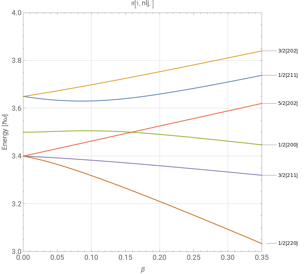
Plot Nilsson Diagram
Plot Nilsson Diagram
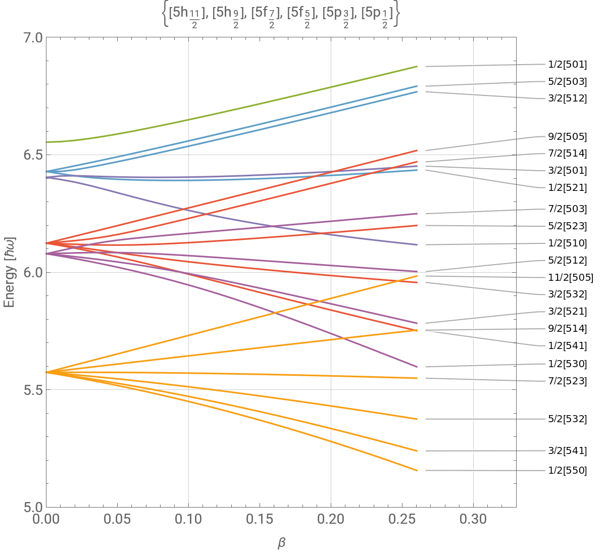
plotYRange={3,4};βRange={0,0.35,0.01};EnergyPlot[H0,Hp,βRange,{βRange〚1;;2〛,plotYRange},Table[If[i28,{Black,Thickness[0.004]},Automatic],{i,1,n}],600,1,1]
color{e1,e2}=Eigensystem[H0];orderIndex=Table[i,{i,1,Length[state]}];j1=e2.orderIndexTable[state〚j1〚i〛〛,{i,1,Length[j1]}]Table[state〚j1〚i〛〛,{i,1,Length[state]}];Table[nn=state〚j1〚i〛,1〛;l=state〚j1〚i〛,2〛;j=state〚j1〚i〛,3〛;Mod[l,2]+2j,{i,1,Length[state]}]gColor=Table[nn=state〚j1〚i〛,1〛;l=state〚j1〚i〛,2〛;j=state〚j1〚i〛,3〛;color〚Mod[Mod[l,2]+2j,Length[color]]+1〛,{i,1,Length[state]}]
,,,,,,,,,,,,,,
{5.,4.,6.,1.,2.,3.}
2,2,,,2,2,,,2,0,,,2,2,,,2,2,,,2,2,,
3
2
1
2
3
2
3
2
1
2
1
2
5
2
5
2
5
2
3
2
5
2
1
2
{3,3,1,5,5,5}
,,,,,
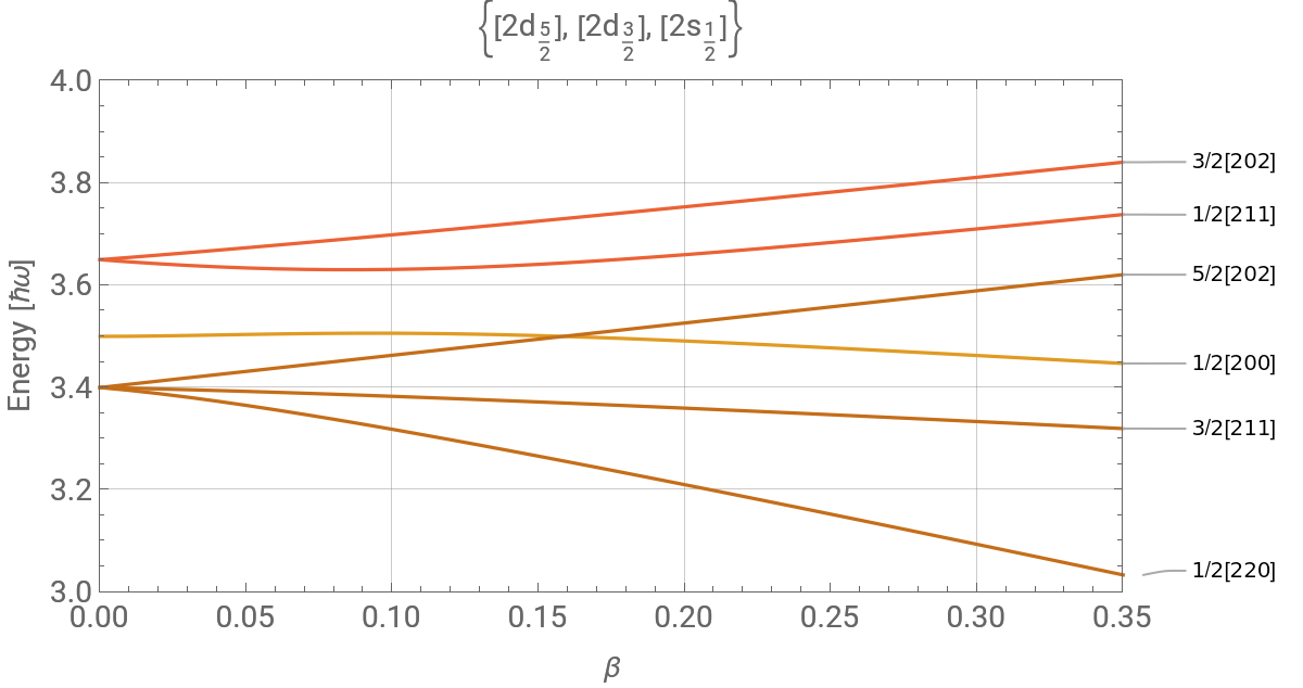
EnergyPlot[H0,Hp,βRange,{βRange〚1;;2〛,plotYRange},gColor,600,0.5,True]
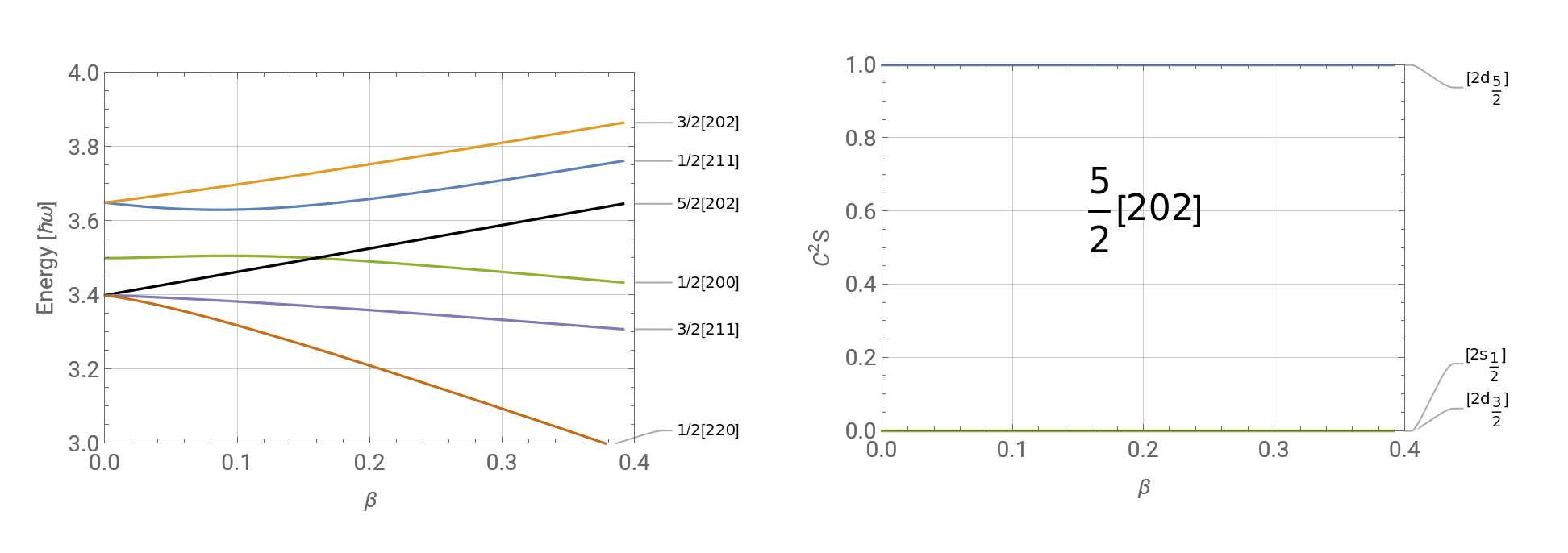
simple output for fixed n - th state
simple output for fixed n - th state
label=Table[Nilsson2[FindStateFromNthState[i,0,H0,Hp]],{i,1,n}];nS=Flatten[Position[label,"5/2[202]"]]〚1〛;βRange=0.0,0.4,0.01;plotYRange={3,4};domS=FindStateFromNthState[nS,0,H0,Hp];TableForm[{domS,StateNLJ[domS],Nilsson[domS]},TableDepth1,TableDirectionsRow](*listandplotofTableofthe*)gg1=EnergyPlot[H0,Hp,βRange,{βRange〚1;;2〛,plotYRange},Table[If[inS,{Black,Thickness[0.005]},Automatic],{i,1,n}],450,0.7,False];gg2=C2SPlot[nS,H0,Hp,βRange,{βRange〚1;;2〛,{0,1}},Table[Style[nlj〚i〛,10],{i,1,Length[nlj]}],450,0.7];GraphicsGrid[{{gg1,gg2}}]TableForm[C2SList[nS,H0,Hp,βRange,2],TableDepth2,TableSpacing{1,4}]
4
3
π
5
2
C
ij
2,2, 5 2 5 2 | 2d 5 2 | 5 2 |
β | δ | Energy | 2d 5 2 | 2d 3 2 | 2s 1 2 |
0. | 0. | 3.4 | 1. | 0 | 0 |
0.0105689 | 0.01 | 3.40667 | 1. | 0 | 0 |
0.0211377 | 0.02 | 3.41333 | 1. | 0 | 0 |
0.0317066 | 0.03 | 3.42 | 1. | 0 | 0 |
0.0422755 | 0.04 | 3.42667 | 1. | 0 | 0 |
0.0528444 | 0.05 | 3.43333 | 1. | 0 | 0 |
0.0634132 | 0.06 | 3.44 | 1. | 0 | 0 |
0.0739821 | 0.07 | 3.44667 | 1. | 0 | 0 |
0.084551 | 0.08 | 3.45333 | 1. | 0 | 0 |
0.0951199 | 0.09 | 3.46 | 1. | 0 | 0 |
0.105689 | 0.1 | 3.46667 | 1. | 0 | 0 |
0.116258 | 0.11 | 3.47333 | 1. | 0 | 0 |
0.126826 | 0.12 | 3.48 | 1. | 0 | 0 |
0.137395 | 0.13 | 3.48667 | 1. | 0 | 0 |
0.147964 | 0.14 | 3.49333 | 1. | 0 | 0 |
0.158533 | 0.15 | 3.5 | 1. | 0 | 0 |
0.169102 | 0.16 | 3.50667 | 1. | 0 | 0 |
0.179671 | 0.17 | 3.51333 | 1. | 0 | 0 |
0.19024 | 0.18 | 3.52 | 1. | 0 | 0 |
0.200809 | 0.19 | 3.52667 | 1. | 0 | 0 |
0.211377 | 0.2 | 3.53333 | 1. | 0 | 0 |
0.221946 | 0.21 | 3.54 | 1. | 0 | 0 |
0.232515 | 0.22 | 3.54667 | 1. | 0 | 0 |
0.243084 | 0.23 | 3.55333 | 1. | 0 | 0 |
0.253653 | 0.24 | 3.56 | 1. | 0 | 0 |
0.264222 | 0.25 | 3.56667 | 1. | 0 | 0 |
0.274791 | 0.26 | 3.57333 | 1. | 0 | 0 |
0.28536 | 0.27 | 3.58 | 1. | 0 | 0 |
0.295928 | 0.28 | 3.58667 | 1. | 0 | 0 |
0.306497 | 0.29 | 3.59333 | 1. | 0 | 0 |
0.317066 | 0.3 | 3.6 | 1. | 0 | 0 |
0.327635 | 0.31 | 3.60667 | 1. | 0 | 0 |
0.338204 | 0.32 | 3.61333 | 1. | 0 | 0 |
0.348773 | 0.33 | 3.62 | 1. | 0 | 0 |
0.359342 | 0.34 | 3.62667 | 1. | 0 | 0 |
0.369911 | 0.35 | 3.63333 | 1. | 0 | 0 |
0.380479 | 0.36 | 3.64 | 1. | 0 | 0 |
0.391048 | 0.37 | 3.64667 | 1. | 0 | 0 |
C2SList[nS,H0,Hp,{0,βRange〚2〛,0.01},1]〚{1,-1}〛//TableForm
β | δ | Energy | 2d 5 2 | 2d 3 2 | 2s 1 2 |
0.4 | 0.37847 | 2.97288 | 0.76459 | -0.341016 | -0.54691 |
K2=Transpose[C2SList[nS,H0,Hp,βRange,2]〚{1,2,12,22,32}〛];K3=K2〚{1,2,3,-1,-2,-3,-4,-5}〛;TableForm[K3,TableDepth2,TableSpacing{1,4}]
β | 0. | 0.105689 | 0.211377 | 0.317066 |
δ | 0. | 0.1 | 0.2 | 0.3 |
Energy | 3.4 | 3.31247 | 3.19696 | 3.07291 |
2s 1 2 | 0 | 0.156752 | 0.246594 | 0.284042 |
2d 3 2 | 0 | 0.017473 | 0.0577747 | 0.0939513 |
2d 5 2 | 1. | 0.825775 | 0.695631 | 0.622007 |
Energy | 3.4 | 3.31247 | 3.19696 | 3.07291 |
δ | 0. | 0.1 | 0.2 | 0.3 |
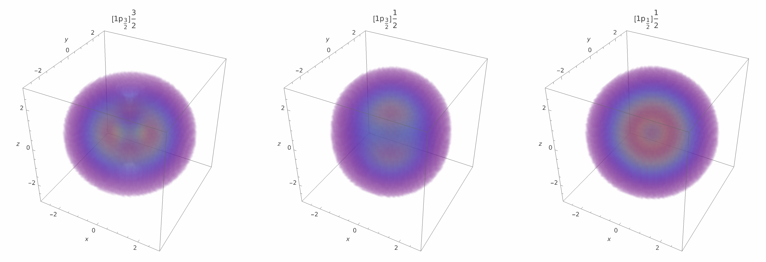
Visualize Orbital
Visualize Orbital
stateFunc1
----+2ArcTan[x,y]+,0,,----+2ArcTan[x,y]+,----z,----+2ArcTan[x,y]+
1
2
2
x
2
y
2
z
2
x
2
y
3/4
π
2---z
1
2
2
x
2
y
2
z
3
3/4
π
1
2
2
x
2
y
2
z
2
x
2
y
3
3/4
π
2
3
1
2
2
x
2
y
2
z
3/4
π
2
3
1
2
2
x
2
y
2
z
2
x
2
y
3/4
π
statestateSstateFunc1=TableΦS++,ArcTanz,+,ArcTan[x,y],statei,{i,1,n}//Simplify;stateFunc2=TableΦS++,ArcTanz,+,-ArcTan[x,y],statei,{i,1,n}//Simplify;stateFunc=Table[stateFunc1〚i〛.stateFunc2〚i〛,{i,1,n}]//SimplifyGraphicsGrid[Partition[Table[DensityPlot3D[stateFunc〚i〛,{x,-3,3},{y,-3,3},{z,-3,3},AxesLabelAutomatic,OpacityFunction0.05,ColorFunction"Rainbow",PlotLabelstateS〚i〛],{i,1,n}],3],ImageSizeFull]
2
x
2
y
2
z
2
x
2
y
2
x
2
y
2
z
2
x
2
y
1,1,,,1,1,,,1,1,,
3
2
3
2
3
2
1
2
1
2
1
2
,,
1p
3
2
3
2
1p
3
2
1
2
1p
1
2
1
2
(+),(++4),
---
2
x
2
y
2
z
2
x
2
y
3/2
π
---
2
x
2
y
2
z
2
x
2
y
2
z
3
3/2
π
2(++)
---
2
x
2
y
2
z
2
x
2
y
2
z
3
3/2
π
{e1,e2}=Eigensystem[H0-0.3Hp];e1e2
2
e2
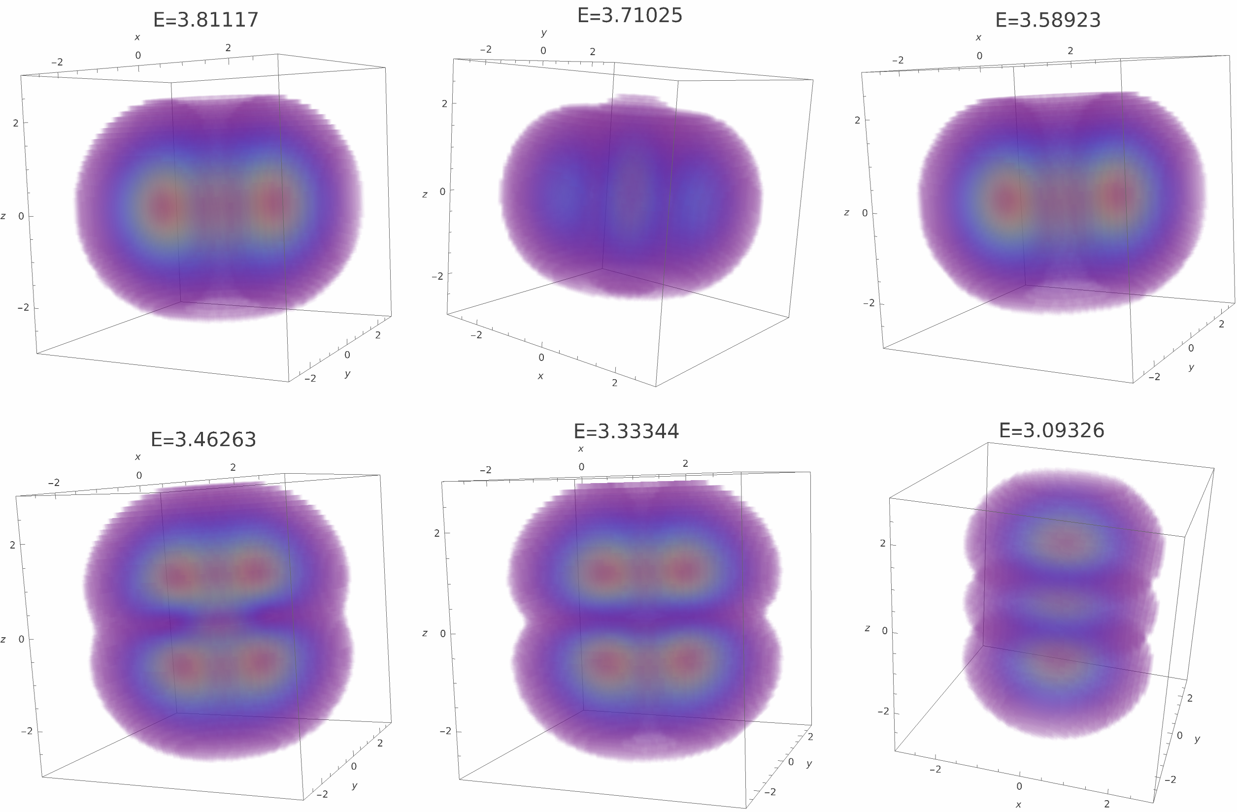
{3.81117,3.71025,3.58923,3.46263,3.33344,3.09326}
{{0.,0.245147,0.,0.969486,0.,0.},{0.,0.,0.278756,0.,-0.595011,0.753828},{1.,0.,0.,0.,0.,0.},{0.,0.,0.539245,0.,0.746496,0.389818},{0.,0.969486,0.,-0.245147,0.,0.},{0.,0.,0.794676,0.,-0.297834,-0.528947}}
{{0.,0.0600971,0.,0.939903,0.,0.},{0.,0.,0.0777049,0.,0.354039,0.568256},{1.,0.,0.,0.,0.,0.},{0.,0.,0.290785,0.,0.557256,0.151958},{0.,0.939903,0.,0.0600971,0.,0.},{0.,0.,0.63151,0.,0.0887049,0.279785}}
stateFuncβ=Table[(e2〚i〛.stateFunc1).(e2〚i〛.stateFunc2),{i,1,n}]//SimplifyGraphicsGrid[Partition[Table[DensityPlot3D[stateFuncβ〚i〛,{x,-3,3},{y,-3,3},{z,-3,3},AxesLabelAutomatic,OpacityFunction0.05,ColorFunction"Rainbow",PlotLabelStyle["E="<>ToString[e1〚i〛],20]],{i,1,n}],3],ImageSizeFull]
(0.0856698+0.0856698+0.0164951+(0.17134+0.0164951)),(0.153077+0.164622+0.164622+0.02267+0.000839327+(-0.31749+0.00558138)+(-0.31749+0.329244+0.00558138)),0.0897936,(0.0409346+0.0147781+0.0147781-0.0653567+0.0260873+(-0.0491909+0.3428)+(-0.0491909+0.0295562+0.3428)),(0.00412376+0.00412376+0.342679+(0.00824753+0.342679)),(0.0753687+0.000186894+0.000186894-0.316488+0.332248+(0.00750626+0.0107928)+(0.00750626+0.000373788+0.0107928))
---
2
x
2
y
2
z
4
x
4
y
2
y
2
z
2
x
2
y
2
z
---
2
x
2
y
2
z
4
x
4
y
2
z
4
z
2
y
2
z
2
x
2
y
2
z
---
2
x
2
y
2
z
2
(+)
2
x
2
y
---
2
x
2
y
2
z
4
x
4
y
2
z
4
z
2
y
2
z
2
x
2
y
2
z
---
2
x
2
y
2
z
4
x
4
y
2
y
2
z
2
x
2
y
2
z
---
2
x
2
y
2
z
4
x
4
y
2
z
4
z
2
y
2
z
2
x
2
y
2
z
Partition[{1,2,3,4,5},3]
{{1,2,3}}
Fitting
Fitting
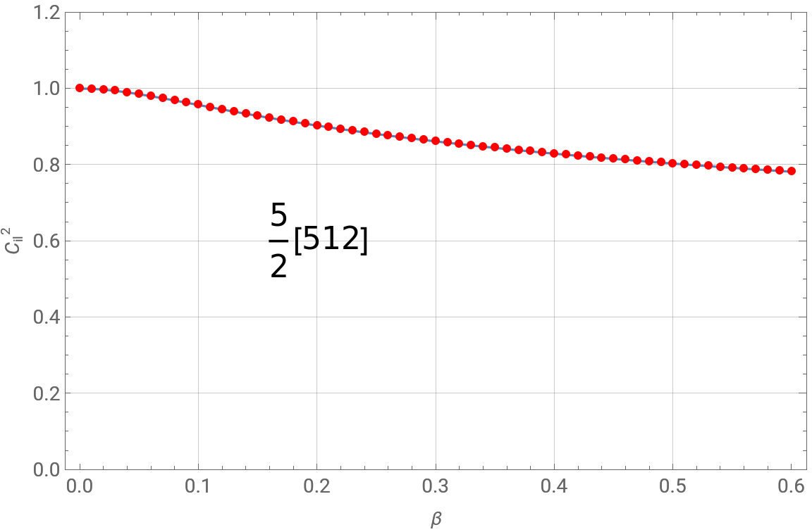
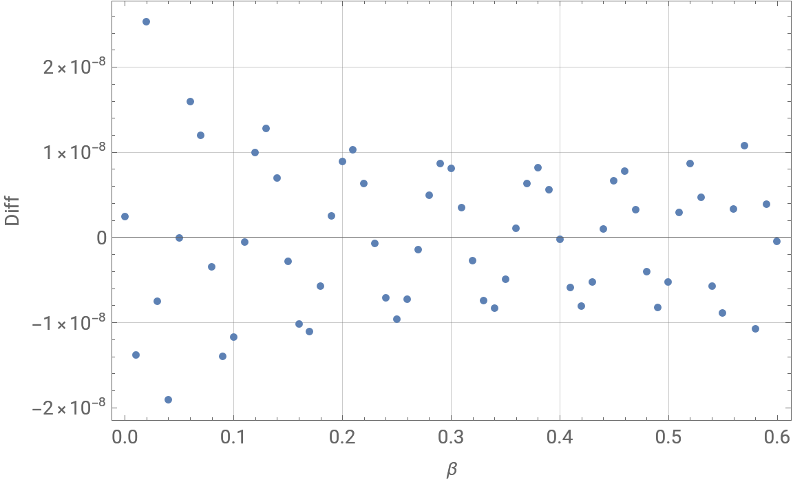
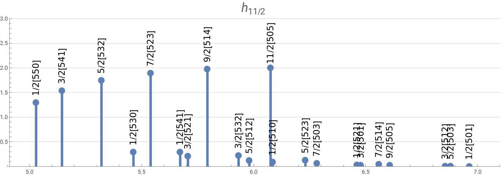
(*needtosetthenljorbitalIndex,checkthenlj,andputthecoulumnnumber*)orbitalIndex=3;βRange={0,0.6,0.01};nljorbital=nlj〚orbitalIndex〛x=Transpose[Transpose[C2SList[nS,H0,Hp,βRange,2]〚2;;-1〛]〚{1,orbitalIndex+2}〛];Length[x]fitX=Fit[x,Table[,{i,0,25}],v]Show[Plot[fitX,{v,βRange〚1〛,βRange〚2〛},PlotRange{All,{0,1.2}},FrameTrue,FrameLabelStyle["β",14],Style["",14],FrameStyle14,GridLinesAutomatic,ImageSizeLarge,PlotLegendsStyle[orbital,22]],ListPlot[x,PlotStyleRed],EpilogText[Style[Nilsson[domS],22],{0.2,0.6}]]dx=Table[{x〚i,1〛,(fitX/.{vx〚i,1〛})-x〚i,2〛},{i,1,Length[x]}];ListPlot[dx,FrameTrue,FrameLabel{Style["β",14],Style["Diff",14]},FrameStyle14,GridLinesAutomatic,ImageSizeLarge]
i
v
2
C
il
,,,,,
5h
11
2
5h
9
2
5f
7
2
5f
5
2
5p
3
2
5p
1
2
5f
7
2
61
1.-0.0000367228v-7.93472+39.0223+111.496-2382.19+11241.3+10059.4-422811.+2.63898×-8.93224×+1.66104×-8.16323×-3.14492×+4.96682×+5.0828×-1.50841×-9.76453×+4.27586×+2.013×-1.2703×-4.22342×+3.96396×-5.9772×+3.8295×-9.56208×
2
v
3
v
4
v
5
v
6
v
7
v
8
v
6
10
9
v
6
10
10
v
7
10
11
v
6
10
12
v
7
10
13
v
7
10
14
v
7
10
15
v
8
10
16
v
7
10
17
v
8
10
18
v
8
10
19
v
9
10
20
v
7
10
21
v
9
10
22
v
9
10
23
v
9
10
24
v
8
10
25
v
 | 5f 7 2 |
single particle energy for fixed deformation
single particle energy for fixed deformation
β=0.3;{e1,e2}=Eigensystem[H0-βHp]//Chop;oi=OrderIndex[β,0.001,H0,Hp]label=Table[Nilsson2[FindStateFromNthState[i,0,H0,Hp]],{i,1,n}]Flatten[Position[label,"1/2[200]"]]〚1〛G3=Table[C2SList[i,H0,Hp,{β,β,0.1},2]〚2,3;;-1〛,{i,1,n}];(*jList=,,,,,;decouple=TableSumjListq+G3i,q+1,{q,1,Length[jList]},{i,1,Length[G3]};G3=Transpose[Join[Transpose[G3],{decouple}]];G4=Join[{Join[{"Energy"},nlj,{"a"}]},G3];*)G4=Join[{Join[{"Energy"},nlj]},G3];G4=Sort[Transpose[Join[{Join[{""},label]},Transpose[G4]]],#1〚2〛>#2〚2〛&];TableForm[G4]TableFormJoin[{"j value of state"},stateJ=DeleteDuplicates[Table[state〚i,3〛,{i,1,n}]]],Join[{"Sum of "},Table[2Sum[G3〚i,j+1〛,{i,1,n}],{j,1,Length[nlj]}]],Join{"SPE for the j-state"},Table,{j,1,Length[nlj]},TableDepth2
11
2
9
2
7
2
5
2
3
2
1
2
jList〚q〛-1/2
(-1)
1
2
2
CS
Sum[e1〚i〛G3〚i,j+1〛,{i,1,n}]
(2stateJ〚j〛+1)/2
{2,1,4,3,5,6}
{1/2[211],3/2[202],1/2[200],5/2[202],3/2[211],1/2[220]}
3
Energy | 2d 5 2 | 2d 3 2 | 2s 1 2 | |
1/2[211] | 3.81117 | 0.0600971 | 0.939903 | 0 |
3/2[202] | 3.71025 | 0.0777049 | 0.354039 | 0.568256 |
1/2[200] | 3.58923 | 1. | 0 | 0 |
5/2[202] | 3.46263 | 0.290785 | 0.557256 | 0.151958 |
3/2[211] | 3.33344 | 0.939903 | 0.0600971 | 0 |
1/2[220] | 3.09326 | 0.63151 | 0.0887049 | 0.279785 |
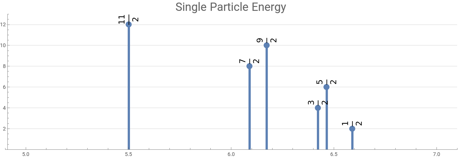
j value of state | 5 2 | 3 2 | 1 2 |
Sum of 2 CS | 6. | 4. | 2. |
SPE for the j-state | 3.4 | 3.65 | 3.5 |
jaja=Table,2Sum[G3〚i,j+1〛,{i,1,n}],{j,1,Length[nlj]}gg1=ListPlotjaja,FillingBottom,FillingStyleThickness[0.005],PlotRange{{4.9,7.1},{0,13}},EpilogTableRotateStyle[Text[stateJ〚i〛,jaja〚i〛+{0,0.5}],14],,{i,1,Length[jaja]},GridLines{{},Automatic},ImageSize800,AspectRatio0.3,PlotLabelStyle["Single Particle Energy",20]
Sum[e1〚i〛G3〚i,j+1〛,{i,1,n}]
(2stateJ〚j〛+1)/2
π
2
{{5.50103,12.},{6.17214,10.},{6.08906,8.},{6.4646,6.},{6.42194,4.},{6.58922,2.}}
Ben' s
Ben' s
βList={0.353,0.326,0.339,0.343,0.348,0.333,0.342,0.338,0.336,0.322,0.326,0.330,0.325,0.254,0.251,0.342,0.338,0.336,0.326,0.330,0.325};oList=Join[Table["1/2[510]",{i,1,15}],Table["5/2[523]",{i,1,6}]]Length[βList]Length[oList]
{1/2[510],1/2[510],1/2[510],1/2[510],1/2[510],1/2[510],1/2[510],1/2[510],1/2[510],1/2[510],1/2[510],1/2[510],1/2[510],1/2[510],1/2[510],5/2[523],5/2[523],5/2[523],5/2[523],5/2[523],5/2[523]}
21
21
label=Table[Nilsson2[FindStateFromNthState[i,0,H0,Hp]],{i,1,n}];Monitor[G3=Table[nS=Flatten[Position[label,oList〚i〛]]〚1〛;C2SList[nS,H0,Hp,{0,βList〚i〛,0.001},2]〚-1〛,{i,1,Length[βList]}],i];
G4=Join[{Join[{"β","δ","Energy"},nlj]},G3];G4=Transpose[Join[{Join[{""},oList]},Transpose[G4]]];TableForm[G4]
β | δ | Energy | 5h 11 2 | 5h 9 2 | 5f 7 2 | 5f 5 2 | 5p 3 2 | 5p 1 2 | |
1/2[510] | 0.353 | 0.334 | 6.06553 | 0.0545908 | 0.279377 | 0.234274 | 0.171409 | 0.0153253 | 0.245023 |
1/2[510] | 0.326 | 0.308453 | 6.07972 | 0.0475486 | 0.271495 | 0.232226 | 0.179009 | 0.021798 | 0.247923 |
1/2[510] | 0.339 | 0.320753 | 6.0728 | 0.0509489 | 0.275505 | 0.233403 | 0.175168 | 0.0184527 | 0.246523 |
1/2[510] | 0.343 | 0.324538 | 6.0707 | 0.051992 | 0.276656 | 0.233691 | 0.174056 | 0.0175116 | 0.246093 |
1/2[510] | 0.348 | 0.329269 | 6.06811 | 0.0532932 | 0.278044 | 0.234006 | 0.172709 | 0.0163896 | 0.245557 |
1/2[510] | 0.333 | 0.315076 | 6.07597 | 0.0493812 | 0.273707 | 0.232907 | 0.176896 | 0.0199405 | 0.247169 |
1/2[510] | 0.342 | 0.323592 | 6.07122 | 0.0517314 | 0.276372 | 0.233622 | 0.174331 | 0.0177432 | 0.2462 |
1/2[510] | 0.338 | 0.319807 | 6.07332 | 0.0506879 | 0.275212 | 0.233325 | 0.175451 | 0.0186942 | 0.24663 |
1/2[510] | 0.336 | 0.317915 | 6.07438 | 0.0501655 | 0.274617 | 0.233164 | 0.176023 | 0.0191849 | 0.246846 |
1/2[510] | 0.322 | 0.304668 | 6.08189 | 0.0465002 | 0.270173 | 0.231785 | 0.180265 | 0.0229217 | 0.248355 |
1/2[510] | 0.326 | 0.308453 | 6.07972 | 0.0475486 | 0.271495 | 0.232226 | 0.179009 | 0.021798 | 0.247923 |
1/2[510] | 0.33 | 0.312238 | 6.07757 | 0.0485962 | 0.272775 | 0.232629 | 0.177788 | 0.02072 | 0.247492 |
1/2[510] | 0.325 | 0.307507 | 6.08026 | 0.0472866 | 0.271169 | 0.232119 | 0.17932 | 0.0220746 | 0.248031 |
1/2[510] | 0.254 | 0.240328 | 6.12215 | 0.0288895 | 0.239319 | 0.216647 | 0.208673 | 0.0511294 | 0.255341 |
1/2[510] | 0.251 | 0.23749 | 6.12411 | 0.0281394 | 0.2375 | 0.215557 | 0.210312 | 0.0528831 | 0.255609 |
5/2[523] | 0.342 | 0.323592 | 6.24425 | 0.0687516 | 0.136187 | 0.783415 | 0.0116467 | 0 | 0 |
5/2[523] | 0.338 | 0.319807 | 6.24204 | 0.0678131 | 0.136964 | 0.783821 | 0.0114023 | 0 | 0 |
5/2[523] | 0.336 | 0.317915 | 6.24094 | 0.0673415 | 0.137361 | 0.784018 | 0.01128 | 0 | 0 |
5/2[523] | 0.326 | 0.308453 | 6.23546 | 0.0649605 | 0.139431 | 0.784941 | 0.0106678 | 0 | 0 |
5/2[523] | 0.33 | 0.312238 | 6.23765 | 0.0659175 | 0.138585 | 0.784585 | 0.0109128 | 0 | 0 |
5/2[523] | 0.325 | 0.307507 | 6.23491 | 0.0647203 | 0.139646 | 0.785027 | 0.0106065 | 0 | 0 |
Export["C_jl.txt",G4]
C_jl.txt
Directory[]
C:\Users\user\Documents
Total[G4〚2,5;;-1〛]
1.
Reproduce Elbek plot
Reproduce Elbek plot
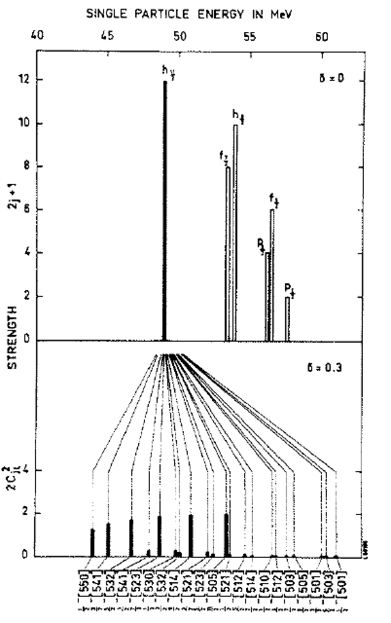
δ=0.3,β=δ{e1,e2}=Eigensystem[H0-βHp]//Chop;oi=OrderIndex[β,0.001,H0,Hp];e1=Table[e1〚oi〚i〛〛,{i,1,Length[e1]}];e2=Table[e2〚oi〚i〛〛,{i,1,Length[e1]}];label=Table[Nilsson2[FindStateFromNthState[i,0,H0,Hp]],{i,1,n}];TableForm[{Table[i,{i,1,Length[stateS]}],stateS}]
4
3
π
5
{0.3,0.317066}
1 | 2 | 3 | 4 | 5 | 6 | 7 | 8 | 9 | 10 | 11 | 12 | 13 | 14 | 15 | 16 | 17 | 18 | 19 | 20 | 21 |
5h 11 2 11 2 | 5h 11 2 9 2 | 5h 11 2 7 2 | 5h 11 2 5 2 | 5h 11 2 3 2 | 5h 11 2 1 2 | 5h 9 2 9 2 | 5h 9 2 7 2 | 5h 9 2 5 2 | 5h 9 2 3 2 | 5h 9 2 1 2 | 5f 7 2 7 2 | 5f 7 2 5 2 | 5f 7 2 3 2 | 5f 7 2 1 2 | 5f 5 2 5 2 | 5f 5 2 3 2 | 5f 5 2 1 2 | 5p 3 2 3 2 | 5p 3 2 1 2 | 5p 1 2 1 2 |
{EnergyPlot[H0,Hp,{0,0.26,0.01},{{0,0.33},{5.0,7.0}},gColor,600,1,True],TableForm[Sort[Transpose[{Table[i,{i,1,Length[e1]}],e1,.stateS}],#1〚2〛>#2〚2〛&]],Sort[Table[{label〚i〛,e1〚i〛,Total[〚i,1;;6〛]},{i,1,Length[e1]}],#1〚2〛>#2〚2〛&]//TableForm}
2
e2
2
e2
 ,
,
,
1 | 6.96186 | 0.171295 5f 5 2 1 2 5f 7 2 1 2 5h 11 2 1 2 5h 9 2 1 2 5p 1 2 1 2 5p 3 2 1 2 |
3 | 6.879 | 0.912887 5f 5 2 5 2 5f 7 2 5 2 5h 11 2 5 2 5h 9 2 5 2 |
4 | 6.85486 | 0.138846 5f 5 2 3 2 5f 7 2 3 2 5h 11 2 3 2 5h 9 2 3 2 5p 3 2 3 2 |
8 | 6.60697 | 0.0113562 5h 11 2 9 2 5h 9 2 9 2 |
9 | 6.55878 | 0.924587 5f 7 2 7 2 5h 11 2 7 2 5h 9 2 7 2 |
5 | 6.47812 | 0.640962 5f 5 2 3 2 5f 7 2 3 2 5h 11 2 3 2 5h 9 2 3 2 5p 3 2 3 2 |
2 | 6.46097 | 0.292087 5f 5 2 1 2 5f 7 2 1 2 5h 11 2 1 2 5h 9 2 1 2 5p 1 2 1 2 5p 3 2 1 2 |
12 | 6.28171 | 0.0423294 5f 7 2 7 2 5h 11 2 7 2 5h 9 2 7 2 |
10 | 6.23059 | 0.0101204 5f 5 2 5 2 5f 7 2 5 2 5h 11 2 5 2 5h 9 2 5 2 |
6 | 6.08459 | 0.181867 5f 5 2 1 2 5f 7 2 1 2 5h 11 2 1 2 5h 9 2 1 2 5p 1 2 1 2 5p 3 2 1 2 |
16 | 6.075 | 1. 5h 11 2 11 2 |
13 | 5.98037 | 0.0742291 5f 5 2 5 2 5f 7 2 5 2 5h 11 2 5 2 5h 9 2 5 2 |
11 | 5.93217 | 2.60067× -6 10 5f 5 2 3 2 5f 7 2 3 2 5h 11 2 3 2 5h 9 2 3 2 5p 3 2 3 2 |
17 | 5.79303 | 0.988644 5h 11 2 9 2 5h 9 2 9 2 |
14 | 5.70614 | 0.21178 5f 5 2 3 2 5f 7 2 3 2 5h 11 2 3 2 5h 9 2 3 2 5p 3 2 3 2 |
7 | 5.67147 | 0.0586853 5f 5 2 1 2 5f 7 2 1 2 5h 11 2 1 2 5h 9 2 1 2 5p 1 2 1 2 5p 3 2 1 2 |
18 | 5.53951 | 0.033084 5f 7 2 7 2 5h 11 2 7 2 5h 9 2 7 2 |
15 | 5.4629 | 0.2877 5f 5 2 1 2 5f 7 2 1 2 5h 11 2 1 2 5h 9 2 1 2 5p 1 2 1 2 5p 3 2 1 2 |
19 | 5.32004 | 0.00276396 5f 5 2 5 2 5f 7 2 5 2 5h 11 2 5 2 5h 9 2 5 2 |
20 | 5.14371 | 0.00840926 5f 5 2 3 2 5f 7 2 3 2 5h 11 2 3 2 5h 9 2 3 2 5p 3 2 3 2 |
21 | 5.02821 | 0.00836527 5f 5 2 1 2 5f 7 2 1 2 5h 11 2 1 2 5h 9 2 1 2 5p 1 2 1 2 5p 3 2 1 2 |
1/2[501] | 6.96186 | 0.00130988 |
5/2[503] | 6.879 | 0.00203921 |
3/2[512] | 6.85486 | 0.00280209 |
9/2[505] | 6.60697 | 0.0113562 |
7/2[514] | 6.55878 | 0.0215604 |
3/2[501] | 6.47812 | 0.0121111 |
1/2[521] | 6.46097 | 0.0150022 |
7/2[503] | 6.28171 | 0.030458 |
5/2[523] | 6.23059 | 0.0628011 |
1/2[510] | 6.08459 | 0.0452063 |
11/2[505] | 6.075 | 1. |
5/2[512] | 5.98037 | 0.0606545 |
3/2[532] | 5.93217 | 0.112008 |
9/2[514] | 5.79303 | 0.988644 |
3/2[521] | 5.70614 | 0.103809 |
1/2[541] | 5.67147 | 0.144861 |
7/2[523] | 5.53951 | 0.947982 |
1/2[530] | 5.4629 | 0.146411 |
5/2[532] | 5.32004 | 0.874505 |
3/2[541] | 5.14371 | 0.76927 |
1/2[550] | 5.02821 | 0.647209 |
haha=Table[{e1〚i〛,Total[2〚i,1;;6〛]},{i,1,Length[e1]}];gg2=ListPlothaha,FillingBottom,FillingStyleThickness[0.005],PlotRange{{4.9,7.1},{0,3}},EpilogTableRotateStyle[Text[label〚i〛,haha〚i〛+{0,0.5}],14],,{i,1,Length[haha]},GridLines{{},Automatic},ImageSize800,AspectRatio0.3,PlotLabelStyle["",20]
2
e2
π
2
h
11/2
Cite this as: Tsz Leung Tang, "Nilsson orbital using perturbation method using spherical harmonic basis" from the Notebook Archive (2020), https://notebookarchive.org/2020-11-an9bzmn
Download
